What is Machine Learning?

What is Machine Learning?

Machine learning can be defined as the science of giving machines an ability to make decisions. The machines are made capable of learning from its own experiences and by analyzing data. Machine learning is a subfield of artificial intelligence. The product of machine learning is an intelligent system, which learns from experience and by finding patterns in data, which is beyond comprehension for humans.

Now machine learning does involve mathematics and computer science, but it differs from the traditional approach. In traditional methods, we explicitly program a computer, give them a set of instructions for a task and the computer use that set of instructions to solve a problem. In machine learning, the computer performs a task without being explicitly programmed. Thus a typical definition of machine learning can be stated as:

“Machine Learning can be defined as the science of making computers act without being explicitly programmed”

In machine learning data is the key, we apply algorithms on data for identifying hidden information in the data i.e what the data is trying to tell us? These identified patterns help the machine learning model to learn and improve its performance.

Machine learning involves mathematics, statistics & computer science.  Statistics helps the model in drawing inferences from the data and to implement an algorithm mathematical equations, process is applied through the means of computer science. Mathematics helps the model evaluate its performance. Machine learning heavily relies on conditions & probability distribution, this is known as modeling. And techniques applied to find appropriate parameters is known as optimization.

Now as I said, machine learning does involve mathematics and computer science but we do not explicitly program a computer using traditional approaches in computation. In machine learning algorithms, we use allow the computer to train itself on data.  A machine learning algorithm will find the most appropriate mathematical relation to define the pattern or trend in data and use that mathematical relation to make predictions on new or unknown data inputs.

Types of Machine Learning

Now we categorize machine learning into three different types of learning. Which is based on the task to perform, available data, & the environment from which our model is expected to gain experience and learn.

Supervised Machine Learning

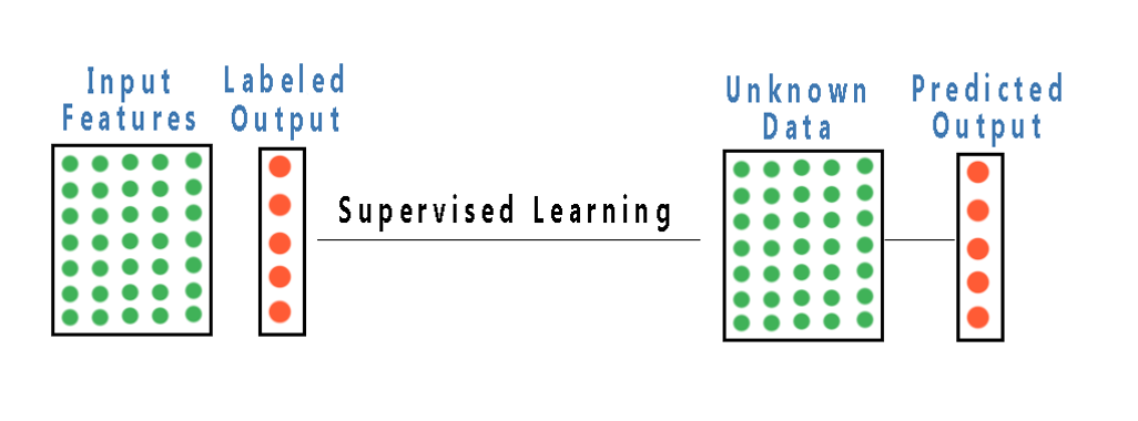First is supervised machine learning: In supervised machine learning, we have a data set which contains the corresponding output labels or results for each input. We call it as our training examples, as our model will learn from these examples. For example, if we want our model to be able to detect the digits in a number, we feed out a model with data containing thousands of images of digits and their corresponding label. Our model learns from these examples and generates a function mapping the inputs to outputs.

The algorithm will learn the relationship between the images and the correct number associated with it, then apply the learning to completely new set of images which it hasn’t seen before and try to predict the correct label. Simply saying in supervised learning we have a set of training examples where input and output are available to us, our model train on the dataset and then try to predict the output of a new unseen data set of similar nature.

Unsupervised Machine Learning

In unsupervised learning the data is unlabeled, that is unlike supervised machine learning here our data set will have no corresponding output variable or target variable, just a bunch of features for a large set of inputs. In unsupervised learning the goal is simple, find the hidden structure or pattern in the data. So in unsupervised learning, we just have a dataset which has no meaning at the beginning and the algorithm will find out the patterns in this dataset which is meaningless to humans.

Let’s consider the example, suppose a bank or financial institution want to detect the customer who is likely to commit a fraud, so the algorithm here will try to find the anomaly in the structure of data. Another example is differentiating the data into different categories, for example recommending movies or products to different categories of customer. Or categorizing the customers based on their spending habits, preference or demographic.

Reinforcement Learning

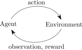
Now reinforcement learning is different. In reinforcement learning, we force the algorithm to learn by experimenting or gaining experience by interacting in an environment. In reinforcement learning, we just leave a learning agent in an environment on its own and it begins to learn with trial and error. For example, a computer learning how to play chess by simply start playing chess, making enormous amounts of errors and using that experience to learn the rules of chess and with regular iterations learn the best chess playing strategies.

Two terms interchangeably used in machine learning domain are data mining and machine learning.  People often get confused between them and they are two different approaches applied for some specific purposes. Let’s study the difference between data mining & machine learning.

• Data mining is the process of identifying hidden patterns in the data aimed to extract important information from the identified structure. It does include techniques of artificial intelligence but the basic purpose is just to identify patterns and not focused on learning from it. Thus data mining may take inspiration from machine learning & mathematics or statistics but is meant for a different purpose. The goal is to use the strength of the various techniques of machine learning and its algorithms to recognize patterns.
• Machine learning is the approach to build artificial intelligence. It is used to develop the new algorithms & techniques allowing a system or machine to learn from the data or from the experience. A system having any type of intelligence must have the ability to learn new knowledge from experiences. So it involves studying algorithms which are able to extract information without human interference.

How does a machine learning algorithm works

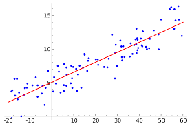
Typically a machine learning task can be described as: learning a mathematical relation that best fits the data. Now let’s suppose we have some random data points with an associated target value as shown in the fig. Now we would like to learn a function which would predict the target value for new input variables. A machine learning algorithm would try to map and learn the function which best describes this given pattern, and then make predictions using that function for new input values.

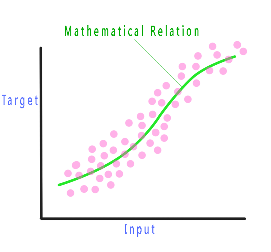
Now let’s suppose looking at the data we assume that the mapping function would look like this line, this is our initial assumption for our final mapping function, we also call it as our initial hypothesis. Now the algorithm will check how closely our hypothesis fits the pattern. It then tries to reduce the error and train itself until it finds the best possible fit. Now depending on the complexity of data there is always a residual error.

Here the algorithm is trying to create a function by mapping the given inputs to its output. This is one way of machine learning, and initially it assumed a basic relationship between the input and output called as our initial hypothesis (which in this case is a line), and this hypothesis helped the algorithm reach the best approximate fit. Depending on the form of our data we make different assumptions about the form it represents and finds a way to optimize that form and generate the best fit. That is why we have a different type of algorithms for different tasks and it is essential to study them and learn when and how to use them.

Initially, we are completely unaware of the form of our mathematical function. So we start with either making an assumption, or we feed the data as it is to the system and let the system decide its form. When an assumption is made about the function, the algorithm applied is called a parametric algorithm and when there is no assumption, the algorithm applied is called non-parametric algorithm. The main difference here is that the parametric algorithm is less expensive in terms of computation, while non-parametric algorithm are computationally expensive and require large data. So we can define a parametric and non-parametric form of learning as:

“A learning model which summarizes the data with a set of fixed size parameters i.e. independent from the number of training examples is known as a parametric model. It doesn’t matter how much data you feed into it, a parametric model won’t change its mind about how many parameters it needs.”

— Artificial Intelligence: A Modern Approach

“Nonparametric methods are good when you have an enormous amount of data and no prior knowledge about it,, and when you don’t want to worry too much about choosing just the right features you go with parametric algorithms.”

— Artificial Intelligence: A Modern Approach

• Low Bias: Less assumptions about the form of the mathematical function.
• High-Bias: Large assumptions about the form of the mathematical function.

Variance is the amount by which the predictions of the learned mathematical function changes if new or different training data was used. Ideally, the predictions should not change too much from one training dataset to the next. It means that the algorithm’s performance is good in identifying the hidden underlying mapping between the inputs and the output variables.

• Low Variance: Small changes in prediction with changes to the training dataset.
• High Variance: Large changes in prediction with changes to the training dataset.

Hence the goal of any learning algorithm is to achieve an optimal balance between bias error & variance error.

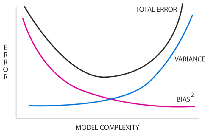
Parametric algorithms often have a high bias but a low variance, while non-parametric or non-linear algorithms often have a low bias but a high variance.

Now as we have gone through a basic introduction to machine learning lets discuss the mathematical processes involved. There is regression analysis & bayesian learning; then there are several non-linear mathematical learning methods, and yes there is slots of calculus.

Regression Analysis

Regression analysis belongs to the field of statistical modeling and is a set of processes for estimating relationship between variables. As you are aware that our dataset is a collection of features or say variables and in supervised machine learning we have a target or output variable, with which our model is supposed to establish a relation and come up with a mathematical function.

The features in our dataset are called as our independent variables and the target feature is called as target variable. Regression analysis helps in understanding how the value of our dependent variable changes when any one of the independent variable varies.

The machine learning model establishes a mathematical function mapping this dependence and that function can represent the variation and structure of our whole data.

And to find the best function, the model goes through an iterative process of eliminating the errors in its prediction and the improving the function on each iteration. The process of eliminating or reducing the errors is done through iterating over a function which calculates the error and each iteration tries to minimize the errors. The most common algorithm used to minimize the errors is the gradient descent algorithm and the most common error function is the ordinary least squares.

Building a regression model means finding the values of the coefficients for our mathematical function to represent our whole data.

1. Simple Linear Regression

In simple linear regression there is a single input feature or variable, and you can easily utilize statistics for estimating the coefficients. It requires you to find the statistical information from the whole data in terms of mean, variation, standard deviation, & covariance.

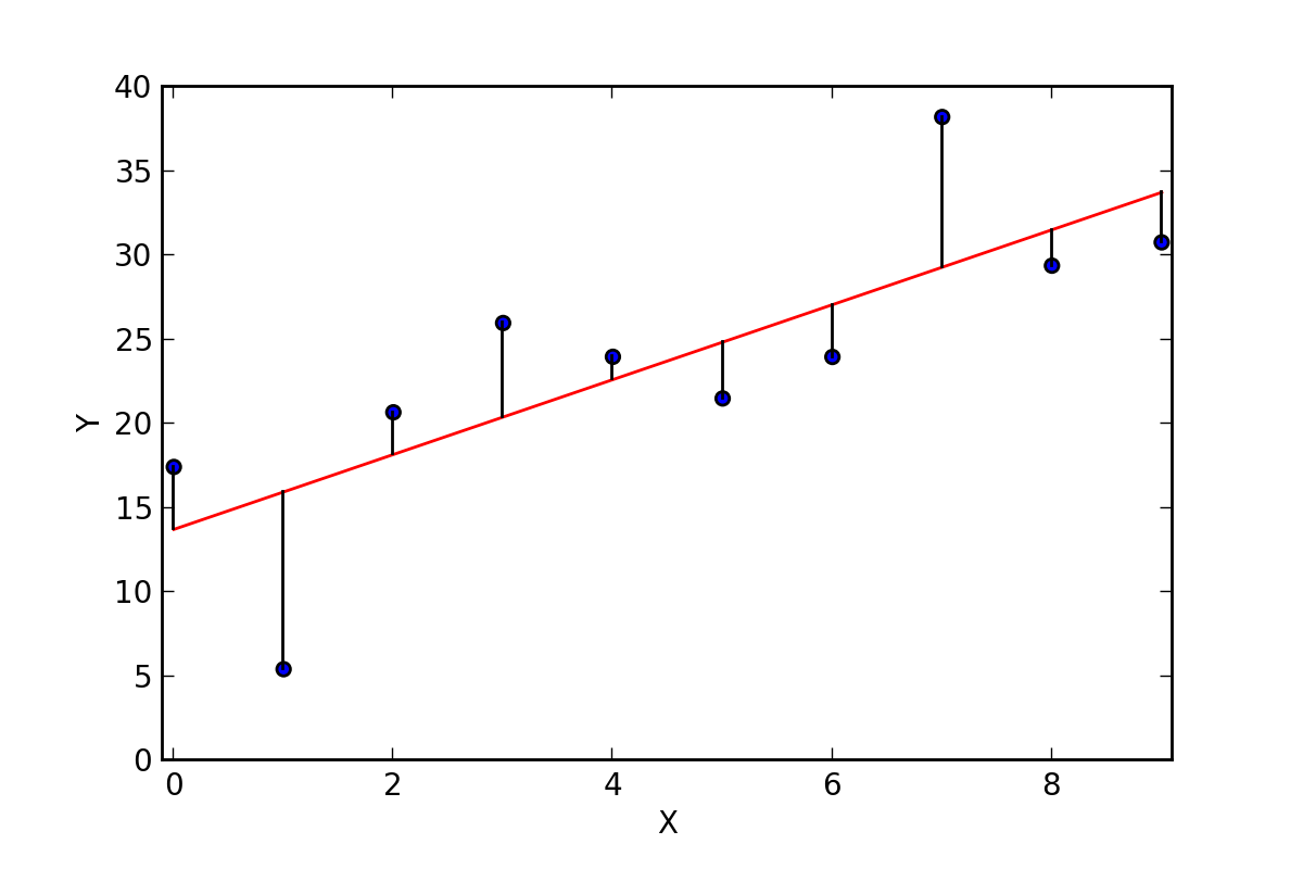
Consider the fig above:

Here the x-axis represent our data point (one dimensional in  this case) and y axis represent the target variable

The equation of the regression line will be then represented by

Y = a₀ + a₁x

This equation is called our initial hypothesis and the algorithm will try to find out the best values for a₀ & a₁ which fits the data with minimum error in prediction

For multiple variables the equation can be written as

Y = a₀ + a₁x + a₂ + . . . . .  + a_nx

These parameters are also called weights due to the fact that they tell us how much weightage a certain variable carries in representation of the data.

2. Ordinary Least Squares

When there are more than one features for our input variables you use Ordinary Least Squares for estimating the coefficients. The Ordinary Least Squares minimize the sum of the squared errors or you can say squared residuals. This means that if we have established a regression line through our data we easily calculate the distance from each data point to our regression line, then we can square it, and then we calculate the sum all of the squared errors. And it is the quantity we need to minimize.

3. Gradient Descent

When we have more than one features as our inputs we can optimize and find the values of our coefficients through going an iterative optimization process of minimizing the error of the model on our data. The technique used is called Gradient Descent and it works by first initiating with some random values for all the coefficient, then the sum of the squared errors are calculated for every pair of input & output variable. We use a learning rate for deciding and setting a speed of the process and it is used as a factor for the amount with which the coefficients will be updated by going in the direction of minimum error. This algorithmic process is iterated until we get a minimum sum of squared error and there is no further improvement possible.

Think of a large bowl in which we usually would eat or put fruit in. This bowl can be represented as a plot of the function we are trying to minimize and it is called the cost function. Any random position on the bowl surface is the value of our current values of the coefficients. The bottom of our bowl is the value for the best set of the coefficients which can minimize the value of our cost function. So the goal here is to repeatedly try and apply different values for the coefficients, calculate the cost and then select new values for the coefficients which gives slightly lower cost. Repeating this will bring the cost to the bottom of our bowl and we will get the values of our most optimal coefficients which provides the minimum cost.

Bayesian Learning

Statistics play a very important role in machine learning, as without logic and probability how will the computer make decisions?

Hence comes the concept of conditional probability which is a part of Bayesian learning

You must have already known about the concept of independent events, where the occurrence of one event does not affect the outcome of another event. Like a coin toss. The probability of independent event is given by

P(A^B) = P(A)*P(B)

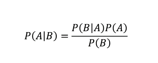
But what about the events where the occurrence of one event affects the other? So here comes the concept of conditional probability, where we can find out the probability of any event which depends on whether another event has occurred or not. For example probability of drawing a king form a deck of card if one king has already been drawn. The conditional probability can be written as:

P(A|B) = P(A and B) / P(B) = P(A∩B) / P(B)

Using this equation you can find out that

Probability of any event A given B has already occurred is given by:

This is our rule and it is the very basic concept which is heavily used in machine learning

The rule involves a very simple derivation which directly comes from the relationship of joint and conditional probabilities. First, notice that the joint probability of A & B both occurring together is given by:
P(A,B) = P(A|B)P(B) = P(B,A) = P(B|A)P(A).

We can rearrange the equation above involving conditional probabilities equal to each other, therefore P(A|B)P(B) = P(B|A)P(A)

and then, divide both sides with P(B) to get the Bayes rule.

In the equation, we want to find the probability of event A, and B is our new information or evidence which is related to A in some way.

P(A|B) is called our posterior i.e the knowledge we get after new information has come to evidence; this is what we are trying to estimate.

P(B|A) is called our likelihood; i.e the probability of getting or observing any new evidence, given our initial hypothesis is true.

P(A) is our prior probability; i.e the probability of our initial hypothesis without the existence of any additional prior knowledge or information.

P(B) is our marginal likelihood; i.e the total probability of getting an evidence.

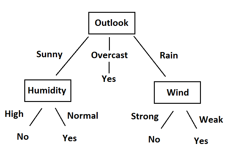
Decision Tree learning

A decision tree is a flowchart like structure in the form of a tree like graph or model. A decision tree forms a tree like structure using nodes and branches, where the first node is the root node and the last nodes are called leaves or terminal nodes which holds the results or outcomes.

Ensemble learning

Ensemble learning methods use multiple algorithms and combine them into one to obtain better predictive performance. Mostly ensemble approaches use a single base learning algorithm to produce multiple homogenous base learners, then create a heterogeneous ensemble. We can also combine heterogeneous learners to create a heterogeneous ensemble.

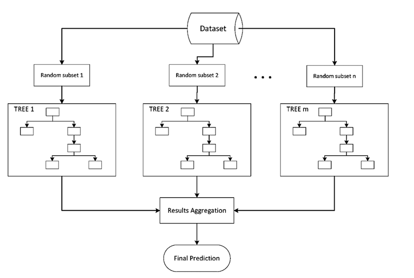
Typically the ensemble are generated sequentially or in parallel. In sequential ensemble the motivation is to exploit the dependence between the base learners i.e we can improve the performance by giving more weightage to previously wrong predictions. In parallel approach the motivation is to exploit the independence between base learners i.e we can reduce the error by taking average of our multiple base learners. Ensemble methods are great for obtaining a balance between bias and variance.

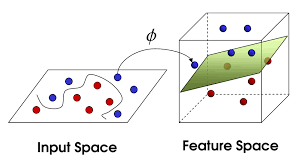
Support Vector Machines

Support vector machine is a supervised Machine learning approach which can be used for both regression and classification. This algorithm is very powerful and can work really well in higher dimensions spaces. They are mostly used for classification problems of high dimensional space and for complex datasets. For a classification problem, the SVM models is a representation of the data as points in n dimensional space. Data is mapped in a way so that separate classification categories are divided by a clear gap that is as wide as possible according to the features. New input is then mapped into the same space and prediction is done by checking on which side of the gap they fall.

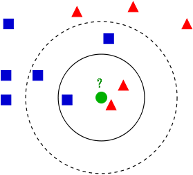
Instance-based learning

So far all the machine learning methods we have discussed constructed a generalized target function for the whole data to build a prediction model. In instance-based learning instead of creating the generalized function new examples are compared with instances in the data. It is called instance-based learning as it constructs a hypothesis directly at the time of estimation from the training examples itself for this approach examples are simply stored and generalization is postponed until a new instance need to be made a prediction on.

Advantage & Disadvantages of Instance-based learning

The advantage of this approach is that even if the target function is too complex and is non-linear in nature, instance-based learning makes the problem decomposable i.e it allows us to create a non-linear function for mapping inputs n outputs. The commonly used instance-based learning algorithm is the K Nearest Neighbors algorithm. The major disadvantage instance-based learning brings is that the need for data increases exponentially with increasing no of features thus making the problem more complex and computationally expensive.

Dimensionality reduction

The machine learning world has a technique of dimensionality reduction where the data having large dimensions is converted into lesser dimensions without losing the information. The data grows exponentially with a number of features so we need to reduce the dimensions for faster computations and helps in memory optimization. The most commonly used algorithm for dimensionality reduction is the Principal Component Analysis algorithm where it projects the higher dimensional data points into lesser dimensional data points without losing any information. Mathematically principal components are Eigenvectors of a covariance matrix.

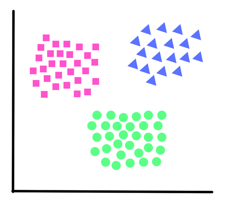
Clustering

in unsupervised learning problems, we do not have an output using which we can generate a target function and generalize our data. We only have data with us with no meaning at first and our task is to find the meantime in it, i.e find the underlying patterns. Clustering can be defined as the task of dividing the population or data points into a number of groups such that data points in same group are similar to each other. Clustering can be categorized into two types hard clustering and soft clustering.

There are several clustering algorithms which can be as follows

Connectivity models: the algorithms are based on the assumption that data points closer in space or more similar these models are easy to interpret but are not scalable for large datasets

Centroid models: it follows an iterative approach by deriving the similarity of data points around a centroid. A dataset can have many centroids according to the problem at hand.

Distribution models: at the names suggest these models work on the principle of how probable is the belonging of a data point to a particular distribution, for example, question Gaussian or binomial distribution.

Density models: These models update the data points and create a cluster for areas of varied density. It just finds different density regions and assigns data points to it.

Deep learning

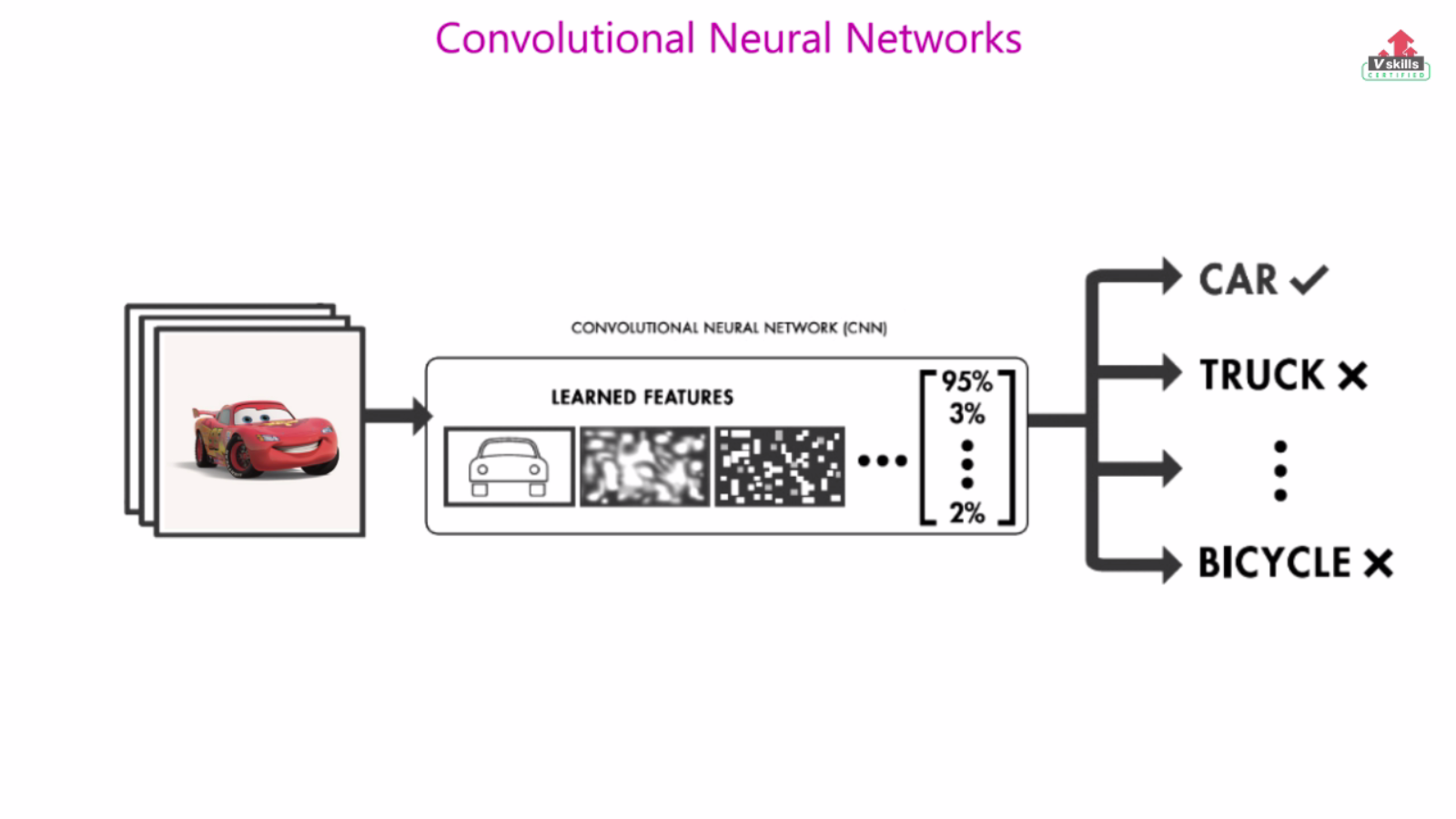
Deep learning is a broader and Deepak aspect of machine learning inspired from human brain particularly from the brain cells called neurons. Deep learning transforms the data into more abstract and composite representations. For example, the data can be an input of images which are represented by a matrix of pixel values, deep learning may learn different aspects and structure from the images, it may learn the abstract which maybe humans cannot perceive, and then use the separate parts to identify structure or objects in new unseen images.

Deep learning is applied to make machines learn more complex structures and perform more complex tasks, like driving a car, flying a helicopter, identify human objects in images or videos and identifying emotion, semantics in language or any form of media.