Major clustering methods can be classified into the following categories.

1. Partitioning methods: Given a database of n objects or data tuples, a partitioning method constructs k partitions of the data, where each partition represents a cluster and k <= n. That is, it classifies the data into k groups, which together satisfy the following requirements: (1) each group must contain at least one object, and (2) each object must belong to exactly one group.

Given k, the number of partitions to construct, a partitioning method creates an initial partitioning. It then uses an iterative relocation technique that attempts to improve the partitioning by moving objects from one group to another. Examples(1) the k-means algorithm and(2) the k-medoids algorithm

2. Hierarchical methods: A hierarchical method creates a hierarchical decomposition of the given set of data objects. A hierarchical method can be classified as being either agglomerative or divisive, based on how the hierarchical decomposition is formed. The agglomerative approach, also called the bottom-up approach, starts with each object forming a separate group. It successively merges the objects or groups that are close to one another, until all of the groups are merged into one (the topmost level of the hierarchy), or  until a termination condition holds. The divisive approach, also called the top-down approach, starts with all of the objects in the same cluster. In each successive iteration, a cluster is split up into smaller clusters, until eventually each object is in one cluster, or until a termination condition holds.

3. Density-based methods: The general idea is to continue growing the given cluster as long as the density  in the “neighborhood” exceeds some threshold. Such a method can be used to filter out noise (outliers) and discover clusters of arbitrary shape.

DBSCAN and its extension, OPTICS, are typical density-based methods.

4. Grid-based methods: Grid-based methods quantize the object space into a finite number of cells that form a grid structure. All of the clustering operations are performed on the grid structure. The main advantage of this approach is its fast processing time, which is typically independent of the number of data objects and dependent only on the number of cells in each dimension in the quantized space.

STING is a typical example of a grid-based method.

5. Model-based methods: Model-based methods hypothesize a model for each of the clusters and find the best fit of the data to the given model. A model-based algorithm may locate clusters by constructing a density function that reflects the spatial distribution of the data points.

6. Clustering high-dimensional data is a particularly important task in cluster analysis

because many applications require the analysis of objects containing a large

number of features or dimensions. As the number of dimensions increases, the

data become increasingly sparse so that the distance measurement between pairs of

points become meaningless and the average density of points anywhere in the data is

likely to be low. Therefore, a different clustering methodology needs to be developed for high-dimensional data. CLIQUE and PROCLUS are two influential subspace clustering methods.

7. Constraint-based clustering is a clustering approach that performs clustering by incorporation of user-specified or application-oriented constraints. A constraint expresses a user’s expectation or describes “properties” of the desired clustering results, and provides an effective means for communicating with the clustering process.

K-means clustering

The k-means algorithm takes the input parameter, k, and partitions a set of n objects into k clusters so that the resulting intracluster similarity is high but the intercluster similarity is low. Cluster similarity is measured in regard to the mean value of the objects in a cluster, which can be viewed as the cluster’s centroid or center of gravity.

The k-means algorithm proceeds as follows:

First, it randomly selects k of the objects, each of which initially represents a cluster mean or center. For each of the remaining objects, an object is assigned to the cluster to which it is the most similar, based on the distance between the object and the cluster mean. It then computes the new mean for each cluster. This process iterates until the criterion function converges. Typically, the square-error criterion is used, defined as

E =i=1kp ∈Ci|p-mi|2

where E is the sum of the square error for all objects in the data set; p is the point in space representing a given object; and mi is the mean of cluster Ci (both p and mi are multidimensional).

Algorithm: 

Input:

1. k: the number of clusters,
2. D: a data set containing n objects.

Output: A set of k clusters.

Method:

(1) arbitrarily choose k objects from D as the initial cluster centers;

(2) repeat

(3) (re)assign each object to the cluster to which the object is the most similar, based on the mean value of the objects in the cluster;

(4) update the cluster means, i.e., calculate the mean value of the objects for each cluster;

(5) until no change;

Advantages:

1. Works well when the clusters are compact clouds that are rather well separated from one another.
2. relatively scalable and efficient in processing.

Limitations:

1. Can be applied only when the mean of a cluster is defined.
2. The necessity for users to specify k in advance can be seen as a disadvantage.
3. Not suitable for discovering clusters with nonconvex shapes or clusters of very different size.
4. Sensitive to noise and outlier data points because a small number of such data can substantially influence the mean value.

Agglomerative clustering

In general, there are two types of hierarchical clustering methods:

1. Agglomerative hierarchical clustering: This bottom-up strategy starts by placing each object in its own cluster and then merges these atomic clusters into larger and larger clusters, until all of the objects are in a single cluster or until certain termination conditions are satisfied. Most hierarchical clustering methods belong to this category.

1. Divisive hierarchical clustering: This top-down strategy does the reverse of agglomerative hierarchical clustering by starting with all objects in one cluster. It subdivides the cluster into smaller and smaller pieces, until each object forms a cluster on its own or until it satisfies certain termination conditions, such as a desired number of clusters is obtained or the diameter of each cluster is within a certain threshold.

2. In either agglomerative or divisive hierarchical clustering, the user can specify the desired number of clusters as a termination condition.

3. A tree structure called a dendrogram is commonly used to represent the process of hierarchical clustering.

Clustering algorithms

Clustering algorithms can be categorized based on their cluster model, as listed above. The following overview will only list the most prominent examples of clustering algorithms, as there are probably a few dozen (if not over 100) published clustering algorithms. Not all provide models for their clusters and can thus not easily be categorized. An overview of algorithms explained in Wikipedia can be found in the list of statistics algorithms.

Connectivity based clustering (hierarchical clustering)

Connectivity based clustering, also known as hierarchical clustering, is based on the core idea of objects being more related to nearby objects than to objects farther away. As such, these algorithms connect "objects" to form "clusters" based on their distance. A cluster can be described largely by the maximum distance needed to connect parts of the cluster. At different distances, different clusters will form, which can be represented using a dendrogram, which explains where the common name "hierarchical clustering" comes from: these algorithms do not provide a single partitioning of the data set, but instead provide an extensive hierarchy of clusters that merge with each other at certain distances. In a dendrogram, the y-axis marks the distance at which the clusters merge, while the objects are placed along the x-axis such that the clusters don't mix.

Connectivity based clustering is a whole family of methods that differ by the way distances are computed. Apart from the usual choice of distance functions, the user also needs to decide on the linkage criterion (since a cluster consists of multiple objects, there are multiple candidates to compute the distance to) to use. Popular choices are known as single-linkage clustering (the minimum of object distances), complete linkage clustering (the maximum of object distances) or UPGMA ("Unweighted Pair Group Method with Arithmetic Mean", also known as average linkage clustering). Furthermore, hierarchical clustering can be agglomerative (starting with single elements and aggregating them into clusters) or divisive (starting with the complete data set and dividing it into partitions).

While these methods are fairly easy to understand, the results are not always easy to use, as they will not produce a unique partitioning of the data set, but a hierarchy the user still needs to choose appropriate clusters from. The methods are not very robust towards outliers, which will either show up as additional clusters or even cause other clusters to merge (known as "chaining phenomenon", in particular with single-linkage clustering). In the general case, the complexity is , which makes them too slow for large data sets. For some special cases, optimal efficient methods (of complexity ) are known: SLINK for single-linkage and CLINK for complete-linkage clustering. In the data mining community these methods are recognized as a theoretical foundation of cluster analysis, but often considered obsolete. They did however provide inspiration for many later methods such as density based clustering.

• Linkage clustering examples
• 

  Single-linkage on Gaussian data. At 35 clusters, the biggest cluster starts fragmenting into smaller parts, while before it was still connected to the second largest due to the single-link effect.

• 

  Single-linkage on density-based clusters. 20 clusters extracted, most of which contain single elements, since linkage clustering does not have a notion of "noise".

Centroid-based clustering

In centroid-based clustering, clusters are represented by a central vector, which may not necessarily be a member of the data set. When the number of clusters is fixed to k, k-means clustering gives a formal definition as an optimization problem: find the cluster centers and assign the objects to the nearest cluster center, such that the squared distances from the cluster are minimized.

The optimization problem itself is known to be NP-hard, and thus the common approach is to search only for approximate solutions. A particularly well known approximative method is Lloyd's algorithm, often actually referred to as "k-means algorithm". It does however only find a local optimum, and is commonly run multiple times with different random initializations. Variations of k-means often include such optimizations as choosing the best of multiple runs, but also restricting the centroids to members of the data set (k-medoids), choosing medians (k-medians clustering), choosing the initial centers less randomly (K-means++) or allowing a fuzzy cluster assignment (Fuzzy c-means).

Most k-means-type algorithms require the number of clusters - - to be specified in advance, which is considered to be one of the biggest drawbacks of these algorithms. Furthermore, the algorithms prefer clusters of approximately similar size, as they will always assign an object to the nearest centroid. This often leads to incorrectly cut borders in between of clusters (which is not surprising, as the algorithm optimized cluster centers, not cluster borders).

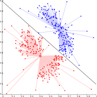
K-means has a number of interesting theoretical properties. On one hand, it partitions the data space into a structure known as Voronoi diagram. On the other hand, it is conceptually close to nearest neighbor classification and as such popular in machine learning. Third, it can be seen as a variation of model based classification, and Lloyd's algorithm as a variation of the Expectation-maximization algorithm for this model discussed below.

• k-Means clustering examples
• 

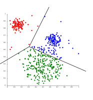
  K-means separates data into Voronoi-cells, which assumes equal-sized clusters (not adequate here)

• 

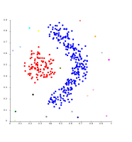
  K-means cannot represent density-based clusters

Distribution-based clustering

The clustering model most closely related to statistics is based on distribution models. Clusters can then easily be defined as objects belonging most likely to the same distribution. A nice property of this approach is that this closely resembles the way artificial data sets are generated: by sampling random objects from a distribution.

While the theoretical foundation of these methods is excellent, they suffer from one key problem known as overfitting, unless constraints are put on the model complexity. A more complex model will usually always be able to explain the data better, which makes choosing the appropriate model complexity inherently difficult.

The most prominent method is known as expectation-maximization algorithm (or short: EM-clustering). Here, the data set is usually modeled with a fixed (to avoid overfitting) number of Gaussian distributions that are initialized randomly and whose parameters are iteratively optimized to fit better to the data set. This will converge to a local optimum, so multiple runs may produce different results. In order to obtain a hard clustering, objects are often then assigned to the Gaussian distribution they most likely belong to, for soft clusterings this is not necessary.

Distribution-based clustering is a semantically strong method, as it not only provides you with clusters, but also produces complex models for the clusters that can also capture correlation and dependence of attributes. However, using these algorithms puts an extra burden on the user: to choose appropriate data models to optimize, and for many real data sets, there may be no mathematical model available the algorithm is able to optimize (e.g. assuming Gaussian distributions is a rather strong assumption on the data).

• EM clustering examples
• 

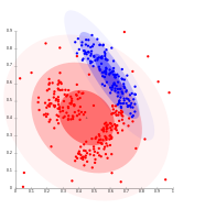
  On Gaussian-distributed data, EM works well, since it uses Gaussians for modelling clusters

• 

  Density-based clusters cannot be modeled using Gaussian distributions

Density-based clustering

In density-based clustering, clusters are defined as areas of higher density than the remainder of the data set. Objects in these sparse areas - that are required to separate clusters - are usually considered to be noise and border points.

The most popular density based clustering method is DBSCAN. In contrast to many newer methods, it features a well-defined cluster model called "density-reachability". Similar to linkage based clustering, it is based on connecting points within certain distance thresholds. However, it only connects points that satisfy a density criterion, in the original variant defined as a minimum number of other objects within this radius. A cluster consists of all density-connected objects (which can form a cluster of an arbitrary shape, in contrast to many other methods) plus all objects that are within these objects' range. Another interesting property of DBSCAN is that its complexity is fairly low - it requires a linear number of range queries on the database - and that it will discover essentially the same results (it is deterministic for core and noise points, but not for border points) in each run, therefore there is no need to run it multiple times. OPTICS is a generalization of DBSCAN that removes the need to choose an appropriate value for the range parameter , and produces a hierarchical result related to that of linkage clustering. DeLi-Clu, Density-Link-Clustering combines ideas from single-linkage clustering and OPTICS, eliminating the parameter entirely and offering performance improvements over OPTICS by using an R-tree index.

The key drawback of DBSCAN and OPTICS is that they expect some kind of density drop to detect cluster borders. Moreover they can not detect intrinsic cluster structures which are prevalent in the majority of real life data. A variation of DBSCAN, EnDBSCAN efficiently detects such kinds of structures. On data sets with, for example, overlapping Gaussian distributions - a common use case in artificial data - the cluster borders produced by these algorithms will often look arbitrary, because the cluster density decreases continuously. On a data set consisting of mixtures of Gaussians, these algorithms are nearly always outperformed by methods such as EM clustering, that are able to precisely model this kind of data.

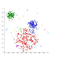
• density-based clustering examples
• 

  Density-based clustering with DBSCAN.

• 

  DBSCAN assumes clusters of similar density, and may have problems separating nearby clusters

• 

  OPTICS is a DBSCAN variant that handles different densities much better