Association Rules Mining

Association rule learning is a popular and well researched method for discovering interesting relations between variables in large databases. Piatetsky-Shapiro describes analyzing and presenting strong rules discovered in databases using different measures of interestingness. Based on the concept of strong rules, Rakesh Agrawal et al. introduced association rules for discovering regularities between products in large-scale transaction data recorded by point-of-sale (POS) systems in supermarkets. For example, the rule  found in the sales data of a supermarket would indicate that if a customer buys onions and potatoes together, he or she is likely to also buy hamburger meat. Such information can be used as the basis for decisions about marketing activities such as, e.g., promotional pricing or product placements. In addition to the above example from market basket analysis association rules are employed today in many application areas including Web usage mining, intrusion detection and bioinformatics. As opposed to sequence mining, association rule learning typically does not consider the order of items either within a transaction or across transactions.
Definition
| transaction ID | milk | bread | butter | beer |
|---|---|---|---|---|
| 1 | 1 | 1 | 0 | 0 |
| 2 | 0 | 0 | 1 | 0 |
| 3 | 0 | 0 | 0 | 1 |
| 4 | 1 | 1 | 1 | 0 |
| 5 | 0 | 1 | 0 | 0 |
Following the original definition by Agrawal et al. the problem of association rule mining is defined as: Let  be a set of
  binary attributes called items. Let
  be a set of transactions called the database. Each transaction in
  has a unique transaction ID and contains a subset of the items in
  . A rule is defined as an implication of the form
  where
where  and
and  . The sets of items (for short itemsets)
  and
and  are called antecedent (left-hand-side or LHS) and consequent (right-hand-side or RHS) of the rule respectively.
To illustrate the concepts, we use a small example from the supermarket domain. The set of items is  and a small database containing the items (1 codes presence and 0 absence of an item in a transaction) is shown in the table to the right. An example rule for the supermarket could be
  meaning that if butter and bread are bought, customers also buy milk.
Note: this example is extremely small. In practical applications, a rule needs a support of several hundred transactions before it can be considered statistically significant, and datasets often contain thousands or millions of transactions.
Useful Concepts
To select interesting rules from the set of all possible rules, constraints on various measures of significance and interest can be used. The best-known constraints are minimum thresholds on support and confidence.
-
The support
 of an itemset is defined as the proportion of transactions in the data set which contain the itemset. In the example database, the itemset
  has a support of
  since it occurs in 20% of all transactions (1 out of 5 transactions).
-
The confidence of a rule is defined
 . For example, the rule
  has a confidence of
  in the database, which means that for 50% of the transactions containing milk and bread the rule is correct (50% of the times a customer buys milk and bread, butter is bought as well). Be careful when reading the expression: here supp(X∪Y) means "support for occurrences of transactions where X and Y both appear", not "support for occurrences of transactions where either X or Y appears", the latter interpretation arising because set union is equivalent to logical disjunction. The argument of
  is a set of preconditions, and thus becomes more restrictive as it grows (instead of more inclusive).
-
Confidence can be interpreted as an estimate of the probability
 , the probability of finding the RHS of the rule in transactions under the condition that these transactions also contain the LHS.
-
The lift of a rule is defined as
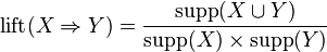 or the ratio of the observed support to that expected if X and Y were independent. The rule has a lift of
  .
.
-
The conviction of a rule is defined as
 . The rule has a conviction of
  , and can be interpreted as the ratio of the expected frequency that X occurs without Y (that is to say, the frequency that the rule makes an incorrect prediction) if X and Y were independent divided by the observed frequency of incorrect predictions. In this example, the conviction value of 1.2 shows that the rule would be incorrect 20% more often (1.2 times as often) if the association between X and Y was purely random chance.
Process

 items. This is called the downward-closure property.
Association rules are usually required to satisfy a user-specified minimum support and a user-specified minimum confidence at the same time. Association rule generation is usually split up into two separate steps:
- First, minimum support is applied to find all frequent itemsets in a database.
- Second, these frequent itemsets and the minimum confidence constraint are used to form rules.
While the second step is straightforward, the first step needs more attention.
Finding all frequent itemsets in a database is difficult since it involves searching all possible itemsets (item combinations). The set of possible itemsets is the power set over and has size  (excluding the empty set which is not a valid itemset). Although the size of the powerset grows exponentially in the number of items in , efficient search is possible using the downward-closure property of support (also called anti-monotonicity) which guarantees that for a frequent itemset, all its subsets are also frequent and thus for an infrequent itemset, all its supersets must also be infrequent. Exploiting this property, efficient algorithms (e.g., Apriori and Eclat) can find all frequent itemsets.
It includes the following topics -
-wikipedia