Topologies and models
There are many types of artificial neural networks (ANN). An artificial neural network is a computational simulation of a biological neural network. These models mimic the real life behaviour of neurons and the electrical messages they produce between input (such as from the eyes or nerve endings in the hand), processing by the brain and the final output from the brain (such as reacting to light or from sensing touch or heat). There are other ANNs which are adaptive systems used to model things such as environments and population.
The systems can be hardware and software based specifically built systems or purely software based and run in computer models.
Feedforward neural network
The feedforward neural network was the first and arguably most simple type of artificial neural network devised. In this network the information moves in only one direction — forwards: From the input nodes data goes through the hidden nodes (if any) and to the output nodes. There are no cycles or loops in the network. Feedforward networks can be constructed from different types of units, e.g. binary McCulloch-Pitts neurons, the simplest example being the perceptron. Continuous neurons, frequently with sigmoidal activation, are used in the context of backpropagation of error.
Radial basis function (RBF) network
Radial basis functions are powerful techniques for interpolation in multidimensional space. A RBF is a function which has built into a distance criterion with respect to a center. Radial basis functions have been applied in the area of neural networks where they may be used as a replacement for the sigmoidal hidden layer transfer characteristic in multi-layer perceptrons. RBF networks have two layers of processing: In the first, input is mapped onto each RBF in the 'hidden' layer. The RBF chosen is usually a Gaussian. In regression problems the output layer is then a linear combination of hidden layer values representing mean predicted output. The interpretation of this output layer value is the same as a regression model in statistics. In classification problems the output layer is typically a sigmoid function of a linear combination of hidden layer values, representing a posterior probability. Performance in both cases is often improved by shrinkage techniques, known as ridge regression in classical statistics and known to correspond to a prior belief in small parameter values (and therefore smooth output functions) in a Bayesian framework.
RBF networks have the advantage of not suffering from local minima in the same way as Multi-Layer Perceptrons. This is because the only parameters that are adjusted in the learning process are the linear mapping from hidden layer to output layer. Linearity ensures that the error surface is quadratic and therefore has a single easily found minimum. In regression problems this can be found in one matrix operation. In classification problems the fixed non-linearity introduced by the sigmoid output function is most efficiently dealt with using iteratively re-weighted least squares.
RBF networks have the disadvantage of requiring good coverage of the input space by radial basis functions. RBF centres are determined with reference to the distribution of the input data, but without reference to the prediction task. As a result, representational resources may be wasted on areas of the input space that are irrelevant to the learning task. A common solution is to associate each data point with its own centre, although this can make the linear system to be solved in the final layer rather large, and requires shrinkage techniques to avoid overfitting.
Associating each input datum with an RBF leads naturally to kernel methods such as support vector machines and Gaussian processes (the RBF is the kernel function). All three approaches use a non-linear kernel function to project the input data into a space where the learning problem can be solved using a linear model. Like Gaussian Processes, and unlike SVMs, RBF networks are typically trained in a Maximum Likelihood framework by maximizing the probability (minimizing the error) of the data under the model. SVMs take a different approach to avoiding overfitting by maximizing instead a margin. RBF networks are outperformed in most classification applications by SVMs. In regression applications they can be competitive when the dimensionality of the input space is relatively small.
Kohonen self-organizing network
The self-organizing map (SOM) invented by Teuvo Kohonen performs a form of unsupervised learning. A set of artificial neurons learn to map points in an input space to coordinates in an output space. The input space can have different dimensions and topology from the output space, and the SOM will attempt to preserve these.
Learning Vector Quantization
Learning Vector Quantization (LVQ) can also be interpreted as a neural network architecture. It was suggested by Teuvo Kohonen, originally. In LVQ, prototypical representatives of the classes parameterize, together with an appropriate distance measure, a distance-based classification scheme.
Recurrent neural network
Contrary to feedforward networks recurrent neural networks (RNNs) are models with bi-directional data flow. While a feedforward network propagates data linearly from input to output, RNNs also propagate data from later processing stages to earlier stages. RNNs can be used as general sequence processors.
Fully recurrent network
This is the basic architecture developed in the 1980s: a network of neuron-like units, each with a directed connection to every other unit. Each unit has a time-varying real-valued activation. Each connection has a modifiable real-valued weight. Some of the nodes are called input nodes, some output nodes, the rest hidden nodes. Most architectures below are special cases.
For supervised learning in discrete time settings, training sequences of real-valued input vectors become sequences of activations of the input nodes, one input vector at a time. At any given time step, each non-input unit computes its current activation as a nonlinear function of the weighted sum of the activations of all units from which it receives connections. There may be teacher-given target activations for some of the output units at certain time steps. For example, if the input sequence is a speech signal corresponding to a spoken digit, the final target output at the end of the sequence may be a label classifying the digit. For each sequence, its error is the sum of the deviations of all target signals from the corresponding activations computed by the network. For a training set of numerous sequences, the total error is the sum of the errors of all individual sequences.
To minimize total error, gradient descent can be used to change each weight in proportion to its derivative with respect to the error, provided the non-linear activation functions are differentiable. Various methods for doing so were developed in the 1980s and early 1990s by Paul Werbos, Ronald J. Williams, Tony Robinson, Jürgen Schmidhuber, Barak Pearlmutter, and others. The standard method is called "backpropagation through time" or BPTT, a generalization of back-propagation for feedforward networks. A more computationally expensive online variant is called "Real-Time Recurrent Learning" or RTRL. Unlike BPTT this algorithm is local in time but not local in space. There also is an online hybrid between BPTT and RTRL with intermediate complexity, and there are variants for continuous time. A major problem with gradient descent for standard RNN architectures is that error gradients vanish exponentially quickly with the size of the time lag between important events, as first realized by Sepp Hochreiter in 1991. The Long short term memory architecture overcomes these problems.
In reinforcement learning settings, there is no teacher providing target signals for the RNN, instead a fitness function or reward function or utility function is occasionally used to evaluate the performance of the RNN, which is influencing its input stream through output units connected to actuators affecting the environment. Variants of evolutionary computation are often used to optimize the weight matrix.
Hopfield network
The Hopfield network (like similar attractor-based networks) is of historic interest although it is not a general RNN, as it is not designed to process sequences of patterns. Instead it requires stationary inputs. It is an RNN in which all connections are symmetric. Invented by John Hopfield in 1982 it guarantees that its dynamics will converge. If the connections are trained using Hebbian learning then the Hopfield network can perform as robust content-addressable memory, resistant to connection alteration.
Boltzmann machine
The Boltzmann machine can be thought of as a noisy Hopfield network. Invented by Geoff Hinton and Terry Sejnowski in 1985, the Boltzmann machine is important because it is one of the first neural networks to demonstrate learning of latent variables (hidden units). Boltzmann machine learning was at first slow to simulate, but the contrastive divergence algorithm of Geoff Hinton (circa 2000) allows models such as Boltzmann machines and Products of Experts to be trained much faster.
Simple recurrent networks
This special case of the basic architecture above was employed by Jeff Elman and Michael I. Jordan. A three-layer network is used, with the addition of a set of "context units" in the input layer. There are connections from the hidden layer (Elman) or from the output layer (Jordan) to these context units fixed with a weight of one. At each time step, the input is propagated in a standard feedforward fashion, and then a simple backprop-like learning rule is applied (this rule is not performing proper gradient descent, however). The fixed back connections result in the context units always maintaining a copy of the previous values of the hidden units (since they propagate over the connections before the learning rule is applied).
Echo state network
The echo state network (ESN) is a recurrent neural network with a sparsely connected random hidden layer. The weights of output neurons are the only part of the network that can change and be trained. ESN are good at reproducing certain time series . A variant for spiking neurons is known as Liquid state machines.
Long short term memory network
The Long short term memory (LSTM), developed by Hochreiter and Schmidhuber in 1997, is an artificial neural net structure that unlike traditional RNNs doesn't have the problem of vanishing gradients. It works even when there are long delays, and it can handle signals that have a mix of low and high frequency components. LSTM RNN outperformed other RNN and other sequence learning methods methods such as HMM in numerous applications such as language learning and connected handwriting recognition.
Bi-directional RNN
Invented by Schuster & Paliwal in 1997 bi-directional RNNs, or BRNNs, use a finite sequence to predict or label each element of the sequence based on both the past and the future context of the element. This is done by adding the outputs of two RNNs: one processing the sequence from left to right, the other one from right to left. The combined outputs are the predictions of the teacher-given target signals. This technique proved to be especially useful when combined with LSTM RNNs.
Hierarchical RNN
There are many instances of hierarchical RNN whose elements are connected in various ways to decompose hierarchical behavior into useful subprograms.
Stochastic neural networks
A stochastic neural network differs from a typical neural network because it introduces random variations into the network. In a probabilistic view of neural networks, such random variations can be viewed as a form of statistical sampling, such as Monte Carlo sampling.
Modular neural networks
Biological studies have shown that the human brain functions not as a single massive network, but as a collection of small networks. This realization gave birth to the concept of modular neural networks, in which several small networks cooperate or compete to solve problems.
Committee of machines
A committee of machines (CoM) is a collection of different neural networks that together "vote" on a given example. This generally gives a much better result compared to other neural network models. Because neural networks suffer from local minima, starting with the same architecture and training but using different initial random weights often gives vastly different networks. A CoM tends to stabilize the result.
The CoM is similar to the general machine learning bagging method, except that the necessary variety of machines in the committee is obtained by training from different random starting weights rather than training on different randomly selected subsets of the training data.
Associative neural network (ASNN)
The ASNN is an extension of the committee of machines that goes beyond a simple/weighted average of different models. ASNN represents a combination of an ensemble of feedforward neural networks and the k-nearest neighbor technique (kNN). It uses the correlation between ensemble responses as a measure of distance amid the analyzed cases for the kNN. This corrects the bias of the neural network ensemble. An associative neural network has a memory that can coincide with the training set. If new data become available, the network instantly improves its predictive ability and provides data approximation (self-learn the data) without a need to retrain the ensemble. Another important feature of ASNN is the possibility to interpret neural network results by analysis of correlations between data cases in the space of models. The method is demonstrated at www.vcclab.org, where it can be used online or downloaded.
Physical neural network
Other types of networks
These special networks do not fit in any of the previous categories.
Holographic associative memory
Holographic associative memory represents a family of analog, correlation-based, associative, stimulus-response memories, where information is mapped onto the phase orientation of complex numbers operating.
Instantaneously trained networks
Instantaneously trained neural networks (ITNNs) were inspired by the phenomenon of short-term learning that seems to occur instantaneously. In these networks the weights of the hidden and the output layers are mapped directly from the training vector data. Ordinarily, they work on binary data, but versions for continuous data that require small additional processing are also available.
Spiking neural networks
Spiking neural networks (SNNs) are models which explicitly take into account the timing of inputs. The network input and output are usually represented as series of spikes (delta function or more complex shapes). SNNs have an advantage of being able to process information in the time domain (signals that vary over time). They are often implemented as recurrent networks. SNNs are also a form of pulse computer.
Spiking neural networks with axonal conduction delays exhibit polychronization, and hence could have a very large memory capacity.
Networks of spiking neurons — and the temporal correlations of neural assemblies in such networks — have been used to model figure/ground separation and region linking in the visual system (see, for example, Reitboeck et al.in Haken and Stadler: Synergetics of the Brain. Berlin, 1989).
In June 2005 IBM announced construction of a Blue Gene supercomputer dedicated to the simulation of a large recurrent spiking neural network.
Gerstner and Kistler have a freely available online textbook on Spiking Neuron Models.
Dynamic neural networks
Dynamic neural networks not only deal with nonlinear multivariate behaviour, but also include (learning of) time-dependent behaviour such as various transient phenomena and delay effects. Techniques to estimate a system process from observed data fall under the general category of system identification.
Cascading neural networks
Cascade Correlation is an architecture and supervised learning algorithm developed by Scott Fahlman and Christian Lebiere. Instead of just adjusting the weights in a network of fixed topology, Cascade-Correlation begins with a minimal network, then automatically trains and adds new hidden units one by one, creating a multi-layer structure. Once a new hidden unit has been added to the network, its input-side weights are frozen. This unit then becomes a permanent feature-detector in the network, available for producing outputs or for creating other, more complex feature detectors. The Cascade-Correlation architecture has several advantages over existing algorithms: it learns very quickly, the network determines its own size and topology, it retains the structures it has built even if the training set changes, and it requires no back-propagation of error signals through the connections of the network.
Neuro-fuzzy networks
A neuro-fuzzy network is a fuzzy inference system in the body of an artificial neural network. Depending on the FIS type, there are several layers that simulate the processes involved in a fuzzy inference like fuzzification, inference, aggregation and defuzzification. Embedding an FIS in a general structure of an ANN has the benefit of using available ANN training methods to find the parameters of a fuzzy system.
Compositional pattern-producing networks
Compositional pattern-producing networks (CPPNs) are a variation of ANNs which differ in their set of activation functions and how they are applied. While typical ANNs often contain only sigmoid functions (and sometimes Gaussian functions), CPPNs can include both types of functions and many others. Furthermore, unlike typical ANNs, CPPNs are applied across the entire space of possible inputs so that they can represent a complete image. Since they are compositions of functions, CPPNs in effect encode images at infinite resolution and can be sampled for a particular display at whatever resolution is optimal.
One-shot associative memory
This type of network can add new patterns without the need for re-training. It is done by creating a specific memory structure, which assigns each new pattern to an orthogonal plane using adjacently connected hierarchical arrays . The network offers real-time pattern recognition and high scalability, it however requires parallel processing and is thus best suited for platforms such as Wireless sensor networks (WSN), Grid computing, and GPGPUs.
Algorithms and Architectures.
The simple Perceptron:
The network adapts as follows: change the weight by an amount proportional to the difference between the desired output and the actual output.
As an equation:
i = η * (D-Y).Ii
where is the learning rate, D is the desired output, and Y is the actual output.
This is called the Perceptron Learning Rule, and goes back to the early 1960's.
We expose the net to the patterns:
| I0 | I1 | Desired output |
|---|---|---|
| 0 | 0 | 0 |
| 0 | 1 | 1 |
| 1 | 0 | 1 |
| 1 | 1 | 1 |
We train the network on these examples. Weights after each epoch (exposure to complete set of patterns) 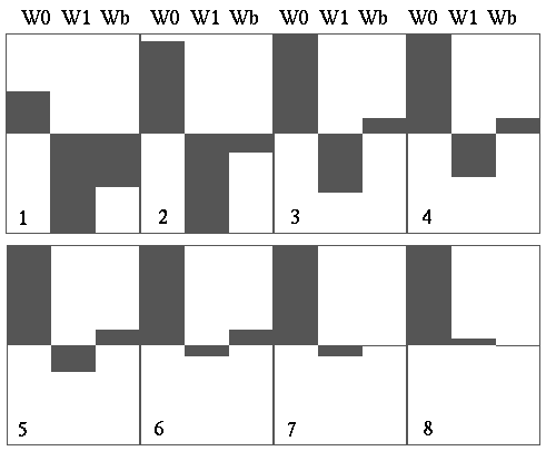
At this point (8) the network has finished learning. Since (D-Y)=0 for all patterns, the weights cease adapting. Single perceptrons are limited in what they can learn:
If we have two inputs, the decision surface is a line. ... and its equation is
1 = (W0/W1).I0 + (Wb/W1)
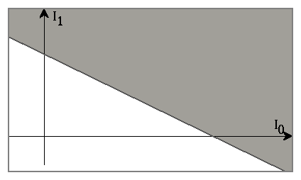
In general, they implement a simple hyperplane decision surface
This restricts the possible mappings available.
Developments from the simple perceptron:
Back-Propagated Delta Rule Networks (BP) (sometimes known and multi-layer perceptrons (MLPs)) and Radial Basis Function Networks (RBF) are both well-known developments of the Delta rule for single layer networks (itself a development of the Perceptron Learning Rule). Both can learn arbitrary mappings or classifications. Further, the inputs (and outputs) can have real values
Back-Propagated Delta Rule Networks (BP)
is a development from the simple Delta rule in which extra hidden layers (layers additional to the input and output layers, not connected externally) are added. The network topology is constrained to be feedforward: i.e. loop-free - generally connections are allowed from the input layer to the first (and possibly only) hidden layer; from the first hidden layer to the second,..., and from the last hidden layer to the output layer.
Typical BP network architecture:
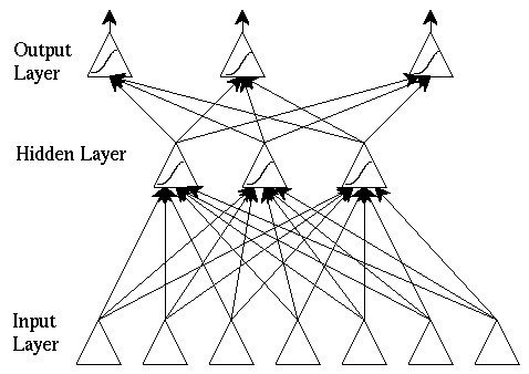
The hidden layer learns to recode (or to provide a representation for) the inputs. More than one hidden layer can be used.
The architecture is more powerful than single-layer networks: it can be shown that any mapping can be learned, given two hidden layers (of units).
The units are a little more complex than those in the original perceptron: their input/output graph is
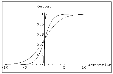
As a function:
in * Xin))
The graph shows the output for k=0.5, 1, and 10, as the activation varies from -10 to 10.
Training BP Networks
The weight change rule is a development of the perceptron learning rule. Weights are changed by an amount proportional to the error at that unit times the output of the unit feeding into the weight.
Running the network consists of
- Forward pass:
- the outputs are calculated and the error at the output units calculated.
- Backward pass:
- The output unit error is used to alter weights on the output units. Then the error at the hidden nodes is calculated (by back-propagating the error at the output units through the weights), and the weights on the hidden nodes altered using these values.
For each data pair to be learned a forward pass and backwards pass is performed. This is repeated over and over again until the error is at a low enough level (or we give up).
Radial Basis function Networks
Radial basis function networks are also feedforward, but have only one hidden layer.
Typical RBF architecture:
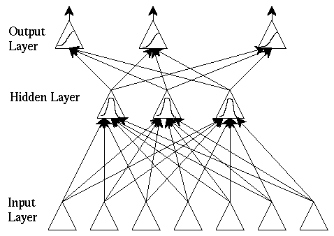
Like BP, RBF nets can learn arbitrary mappings: the primary difference is in the hidden layer.
RBF hidden layer units have a receptive field which has a centre: that is, a particular input value at which they have a maximal output.Their output tails off as the input moves away from this point.
Generally, the hidden unit function is a Gaussian:
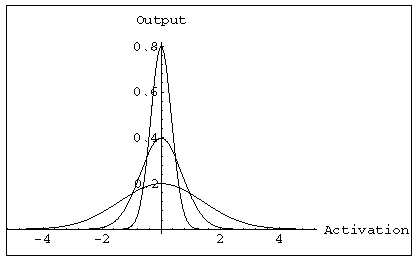
Gaussians with three different standard deviations.
Training RBF Networks.
RBF networks are trained by
- deciding on how many hidden units there should be
- deciding on their centres and the sharpnesses (standard deviation) of their Gaussians
- training up the output layer.
Generally, the centres and SDs are decided on first by examining the vectors in the training data. The output layer weights are then trained using the Delta rule. BP is the most widely applied neural network technique. RBFs are gaining in popularity.
Nets can be
- trained on classification data (each output represents one class), and then used directly as classifiers of new data.
- trained on (x,f(x)) points of an unknown function f, and then used to interpolate.
RBFs have the advantage that one can add extra units with centres near parts of the input which are difficult to classify. Both BP and RBFs can also be used for processing time-varying data: one can consider a window on the data:
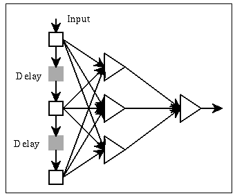
Networks of this form (finite-impulse response) have been used in many applications.
There are also networks whose architectures are specialised for processing time-series.
Unsupervised networks:
Simple Perceptrons, BP, and RBF networks need a teacher to tell the network what the desired output should be. These are supervised networks.
In an unsupervised net, the network adapts purely in response to its inputs. Such networks can learn to pick out structure in their input.
Applications for unsupervised nets
- clustering data:
- exactly one of a small number of output units comes on in response to an input.
- reducing the dimensionality of data:
- data with high dimension (a large number of input units) is compressed into a lower dimension (small number of output units).
Although learning in these nets can be slow, running the trained net is very fast - even on a computer simulation of a neural net.
Kohonen clustering Algorithm:
- takes a high-dimensional input, and clusters it, but retaining some topological ordering of the output.
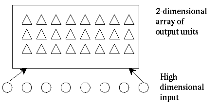
After training, an input will cause some the output units in some area to become active.
Such clustering (and dimensionality reduction) is very useful as a preprocessing stage, whether for further neural network data processing, or for more traditional techniques.
-Stirling university, wikipedia

