FUZZY LOGIC

The concept of Fuzzy Logic (FL) was conceived by Lotfi Zadeh, a professor at the University of California at Berkley, and presented not as a control methodology, but as a way of processing data by allowing partial set membership rather than crisp set membership or non-membership. This approach to set theory was not applied to control systems until the 70's due to insufficient small-computer capability prior to that time. Professor Zadeh reasoned that people do not require precise, numerical information input, and yet they are capable of highly adaptive control. If feedback controllers could be programmed to accept noisy, imprecise input, they would be much more effective and perhaps easier to implement. Unfortunately, U.S. manufacturers have not been so quick to embrace this technology while the Europeans and Japanese have been aggressively building real products around it.

In this context, FL is a problem-solving control system methodology that lends itself to implementation in systems ranging from simple, small, embedded micro-controllers to large, networked, multi-channel PC or workstation-based data acquisition and control systems. It can be implemented in hardware, software, or a combination of both. FL provides a simple way to arrive at a definite conclusion based upon vague, ambiguous, imprecise, noisy, or missing input information. FL's approach to control problems mimics how a person would make decisions, only much faster.

FL incorporates a simple, rule-based IF X AND Y THEN Z approach to a solving control problem rather than attempting to model a system mathematically. The FL model is empirically-based, relying on an operator's experience rather than their technical understanding of the system. For example, rather than dealing with temperature control in terms such as "SP =500F", "T <1000F", or "210C
FL WORKING
FL requires some numerical parameters in order to operate such as what is considered significant error and significant rate-of-change-of-error, but exact values of these numbers are usually not critical unless very responsive performance is required in which case empirical tuning would determine them. For example, a simple temperature control system could use a single temperature feedback sensor whose data is subtracted from the command signal to compute "error" and then time-differentiated to yield the error slope or rate-of-change-of-error, hereafter called "error-dot". Error might have units of degs F and a small error considered to be 2F while a large error is 5F. The "error-dot" might then have units of degs/min with a small error-dot being 5F/min and a large one being 15F/min. These values don't have to be symmetrical and can be "tweaked" once the system is operating in order to optimize performance. Generally, FL is so forgiving that the system will probably work the first time without any tweaking.


FL USE
FL offers several unique features that make it a particularly good choice for many control problems.
1) It is inherently robust since it does not require precise, noise-free inputs and can be programmed to fail safely if a feedback sensor quits or is destroyed. The output control is a smooth control function despite a wide range of input variations.
2) Since the FL controller processes user-defined rules governing the target control system, it can be modified and tweaked easily to improve or drastically alter system performance. New sensors can easily be incorporated into the system simply by generating appropriate governing rules.
3) FL is not limited to a few feedback inputs and one or two control outputs, nor is it necessary to measure or compute rate-of-change parameters in order for it to be implemented. Any sensor data that provides some indication of a system's actions and reactions is sufficient. This allows the sensors to be inexpensive and imprecise thus keeping the overall system cost and complexity low.
4) Because of the rule-based operation, any reasonable number of inputs can be processed (1-8 or more) and numerous outputs (1-4 or more) generated, although defining the rulebase quickly becomes complex if too many inputs and outputs are chosen for a single implementation since rules defining their interrelations must also be defined. It would be better to break the control system into smaller chunks and use several smaller FL controllers distributed on the system, each with more limited responsibilities.
5) FL can control nonlinear systems that would be difficult or impossible to model mathematically. This opens doors for control systems that would normally be deemed unfeasible for automation.

FL USAGE
1) Define the control objectives and criteria: What am I trying to control? What do I have to do to control the system? What kind of response do I need? What are the possible (probable) system failure modes?
2) Determine the input and output relationships and choose a minimum number of variables for input to the FL engine (typically error and rate-of-change-of-error).
3) Using the rule-based structure of FL, break the control problem down into a series of IF X AND Y THEN Z rules that define the desired system output response for given system input conditions. The number and complexity of rules depends on the number of input parameters that are to be processed and the number fuzzy variables associated with each parameter. If possible, use at least one variable and its time derivative. Although it is possible to use a single, instantaneous error parameter without knowing its rate of change, this cripples the system's ability to minimize overshoot for a step inputs.
4) Create FL membership functions that define the meaning (values) of Input/Output terms used in the rules.
5) Create the necessary pre- and post-processing FL routines if implementing in S/W, otherwise program the rules into the FL H/W engine.
6) Test the system, evaluate the results, tune the rules and membership functions, and retest until satisfactory results are obtained.

LINGUISTIC VARIABLES
In 1973, Professor Lotfi Zadeh proposed the concept of linguistic or "fuzzy" variables. Think of them as linguistic objects or words, rather than numbers. The sensor input is a noun, e.g. "temperature", "displacement", "velocity", "flow", "pressure", etc. Since error is just the difference, it can be thought of the same way. The fuzzy variables themselves are adjectives that modify the variable (e.g. "large positive" error, "small positive" error ,"zero" error, "small negative" error, and "large negative" error). As a minimum, one could simply have "positive", "zero", and "negative" variables for each of the parameters. Additional ranges such as "very large" and "very small" could also be added to extend the responsiveness to exceptional or very nonlinear conditions, but aren't necessary in a basic system.

THE RULE MATRIX
The fuzzy parameters of error (command-feedback) and error-dot (rate-of-change-of-error) were modified by the adjectives "negative", "zero", and "positive". To picture this, imagine the simplest practical implementation, a 3-by-3 matrix. The columns represent "negative error", "zero error", and "positive error" inputs from left to right. The rows represent "negative", "zero", and "positive" "error-dot" input from top to bottom. This planar construct is called a rule matrix. It has two input conditions, "error" and "error-dot", and one output response conclusion (at the intersection of each row and column). In this case there are nine possible logical product (AND) output response conclusions.

Although not absolutely necessary, rule matrices usually have an odd number of rows and columns to accommodate a "zero" center row and column region. This may not be needed as long as the functions on either side of the center overlap somewhat and continuous dithering of the output is acceptable since the "zero" regions correspond to "no change" output responses the lack of this region will cause the system to continually hunt for "zero". It is also possible to have a different number of rows than columns. This occurs when numerous degrees of inputs are needed. The maximum number of possible rules is simply the product of the number of rows and columns, but definition of all of these rules may not be necessary since some input conditions may never occur in practical operation. The primary objective of this construct is to map out the universe of possible inputs while keeping the system sufficiently under control.

MEMBERSHIP FUNCTIONS
The membership function is a graphical representation of the magnitude of participation of each input. It associates a weighting with each of the inputs that are processed, define functional overlap between inputs, and ultimately determines an output response. The rules use the input membership values as weighting factors to determine their influence on the fuzzy output sets of the final output conclusion. Once the functions are inferred, scaled, and combined, they are defuzzified into a crisp output which drives the system. There are different membership functions associated with each input and output response. Some features to note are:

SHAPE - triangular is common, but bell, trapezoidal, haversine and, exponential have been used. More complex functions are possible but require greater computing overhead to implement.. HEIGHT or magnitude (usually normalized to 1) WIDTH (of the base of function), SHOULDERING (locks height at maximum if an outer function. Shouldered functions evaluate as 1.0 past their center) CENTER points (center of the member function shape) OVERLAP (N&Z, Z&P, typically about 50% of width but can be less).

INFERENCING
The MAX-MIN method tests the magnitudes of each rule and selects the highest one. The horizontal coordinate of the "fuzzy centroid" of the area under that function is taken as the output. This method does not combine the effects of all applicable rules but does produce a continuous output function and is easy to implement.

The MAX-DOT or MAX-PRODUCT method scales each member function to fit under its respective peak value and takes the horizontal coordinate of the "fuzzy" centroid of the composite area under the function(s) as the output. Essentially, the member function(s) are shrunk so that their peak equals the magnitude of their respective function ("negative", "zero", and "positive"). This method combines the influence of all active rules and produces a smooth, continuous output.

The AVERAGING method is another approach that works but fails to give increased weighting to more rule votes per output member function. For example, if three "negative" rules fire, but only one "zero" rule does, averaging will not reflect this difference since both averages will equal 0.5. Each function is clipped at the average and the "fuzzy" centroid of the composite area is computed.

The ROOT-SUM-SQUARE (RSS) method combines the effects of all applicable rules, scales the functions at their respective magnitudes, and computes the "fuzzy" centroid of the composite area. This method is more complicated mathematically than other methods, but was selected for this example since it seemed to give the best weighted influence to all firing rules.

Fuzzy logic allows for approximate values and inferences as well as incomplete or ambiguous data (fuzzy data) as opposed to only relying on crisp data (binary yes/no choices).

Degrees of truth

Fuzzy logic and probabilistic logic are mathematically similar – both have truth values ranging between 0 and 1 – but conceptually distinct, owing to different interpretations—see interpretations of probability theory. Fuzzy logic corresponds to "degrees of truth", while probabilistic logic corresponds to "probability, likelihood"; as these differ, fuzzy logic and probabilistic logic yield different models of the same real-world situations.

Both degrees of truth and probabilities range between 0 and 1 and hence may seem similar at first. For example, let a 100  ml glass contain 30 ml of water. Then we may consider two concepts: Empty and Full. The meaning of each of them can be represented by a certain fuzzy set. Then one might define the glass as being 0.7 empty and 0.3 full. Note that the concept of emptiness would be subjective and thus would depend on the observer or designer. Another designer might equally well design a set membership function where the glass would be considered full for all values down to 50 ml. It is essential to realize that fuzzy logic uses truth degrees as a mathematical model of the vagueness phenomenon while probability is a mathematical model of ignorance.

Applying truth values

A basic application might characterize subranges of a continuous variable. For instance, a temperature measurement for anti-lock brakes might have several separate membership functions defining particular temperature ranges needed to control the brakes properly. Each function maps the same temperature value to a truth value in the 0 to 1 range. These truth values can then be used to determine how the brakes should be controlled.

Fuzzy logic temperature

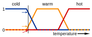
In this image, the meanings of the expressions cold, warm, and hot are represented by functions mapping a temperature scale. A point on that scale has three "truth values"—one for each of the three functions. The vertical line in the image represents a particular temperature that the three arrows (truth values) gauge. Since the red arrow points to zero, this temperature may be interpreted as "not hot". The orange arrow (pointing at 0.2) may describe it as "slightly warm" and the blue arrow (pointing at 0.8) "fairly cold".

Linguistic variables

While variables in mathematics usually take numerical values, in fuzzy logic applications, the non-numeric linguistic variables are often used to facilitate the expression of rules and facts.

A linguistic variable such as age may have a value such as young or its antonym old. However, the great utility of linguistic variables is that they can be modified via linguistic hedges applied to primary terms. The linguistic hedges can be associated with certain functions.

Example

Fuzzy set theory defines fuzzy operators on fuzzy sets. The problem in applying this is that the appropriate fuzzy operator may not be known. For this reason, fuzzy logic usually uses IF-THEN rules, or constructs that are equivalent, such as fuzzy associative matrices.

Rules are usually expressed in the form:
IF variable IS property THEN action

For example, a simple temperature regulator that uses a fan might look like this:

IF temperature IS very cold THEN stop fan
IF temperature IS cold THEN turn down fan
IF temperature IS normal THEN maintain level
IF temperature IS hot THEN speed up fan

There is no "ELSE" – all of the rules are evaluated, because the temperature might be "cold" and "normal" at the same time to different degrees.

The AND, OR, and NOT operators of boolean logic exist in fuzzy logic, usually defined as the minimum, maximum, and complement; when they are defined this way, they are called the Zadeh operators. So for the fuzzy variables x and y:

NOT x = (1 - truth(x))
x AND y = minimum(truth(x), truth(y))
x OR y = maximum(truth(x), truth(y))

There are also other operators, more linguistic in nature, called hedges that can be applied. These are generally adverbs such as "very", or "somewhat", which modify the meaning of a set using a mathematical formula.

Neural Network

An Artificial Neural Network, often just called a neural network, is a mathematical model inspired by biological neural networks. A neural network consists of an interconnected group of artificial neurons, and it processes information using a connectionist approach to computation. In most cases a neural network is an adaptive system that changes its structure during a learning phase. Neural networks are used to model complex relationships between inputs and outputs or to find patterns in data.

The inspiration for neural networks came from examination of central nervous systems. In an artificial neural network, simple artificial nodes, called "neurons", "neurodes", "processing elements" or "units", are connected together to form a network which mimics a biological neural network.

There is no single formal definition of what an artificial neural network is. Generally, it involves a network of simple processing elements that exhibit complex global behavior determined by the connections between the processing elements and element parameters. Artificial neural networks are used with algorithms designed to alter the strength of the connections in the network to produce a desired signal flow.

Neural networks are also similar to biological neural networks in that functions are performed collectively and in parallel by the units, rather than there being a clear delineation of subtasks to which various units are assigned. The term "neural network" usually refers to models employed in statistics, cognitive psychology and artificial intelligence. Neural network models which emulate the central nervous system are part of theoretical neuroscience and computational neuroscience.

In modern software implementations of artificial neural networks, the approach inspired by biology has been largely abandoned for a more practical approach based on statistics and signal processing. In some of these systems, neural networks or parts of neural networks (such as artificial neurons) are used as components in larger systems that combine both adaptive and non-adaptive elements. While the more general approach of such adaptive systems is more suitable for real-world problem solving, it has far less to do with the traditional artificial intelligence connectionist models. What they do have in common, however, is the principle of non-linear, distributed, parallel and local processing and adaptation. Historically, the use of neural networks models marked a paradigm shift in the late eighties from high-level (symbolic) artificial intelligence, characterized by expert systems with knowledge embodied in if-then rules, to low-level (sub-symbolic) machine learning, characterized by knowledge embodied in the parameters of a dynamical system.

Applications

The utility of artificial neural network models lies in the fact that they can be used to infer a function from observations. This is particularly useful in applications where the complexity of the data or task makes the design of such a function by hand impractical.

Real-life applications

The tasks artificial neural networks are applied to tend to fall within the following broad categories:

• Function approximation, or regression analysis, including time series prediction, fitness approximation and modeling.
• Classification, including pattern and sequence recognition, novelty detection and sequential decision making.
• Data processing, including filtering, clustering, blind source separation and compression.
• Robotics, including directing manipulators, Computer numerical control.

Application areas include system identification and control (vehicle control, process control, natural resources management), quantum chemistry, game-playing and decision making (backgammon, chess, poker), pattern recognition (radar systems, face identification, object recognition and more), sequence recognition (gesture, speech, handwritten text recognition), medical diagnosis, financial applications (automated trading systems), data mining (or knowledge discovery in databases, "KDD"), visualization and e-mail spam filtering.

Artificial neural networks have also been used to diagnose several cancers. An ANN based hybrid lung cancer detection system named HLND improves the accuracy of diagnosis and the speed of lung cancer radiology. These networks have also been used to diagnose prostate cancer. The diagnoses can be used to make specific models taken from a large group of patients compared to information of one given patient. The models do not depend on assumptions about correlations of different variables. Colorectal cancer has also been predicted using the neural networks. Neural networks could predict the outcome for a patient with colorectal cancer with a lot more accuracy than the current clinical methods. After training, the networks could predict multiple patient outcomes from unrelated institutions.

Neural networks and neuroscience

Theoretical and computational neuroscience is the field concerned with the theoretical analysis and computational modeling of biological neural systems. Since neural systems are intimately related to cognitive processes and behavior, the field is closely related to cognitive and behavioral modeling.

The aim of the field is to create models of biological neural systems in order to understand how biological systems work. To gain this understanding, neuroscientists strive to make a link between observed biological processes (data), biologically plausible mechanisms for neural processing and learning (biological neural network models) and theory (statistical learning theory and information theory).

There are many types of artificial neural networks (ANN). An artificial neural network is a computational simulation of a biological neural network. These models mimic the real life behaviour of neurons and the electrical messages they produce between input (such as from the eyes or nerve endings in the hand), processing by the brain and the final output from the brain (such as reacting to light or from sensing touch or heat). There are other ANNs which are adaptive systems used to model things such as environments and population.

The systems can be hardware and software based specifically built systems or purely software based and run in computer models.

Feedforward neural network

The feedforward neural network was the first and arguably most simple type of artificial neural network devised. In this network the information moves in only one direction — forwards: From the input nodes data goes through the hidden nodes (if any) and to the output nodes. There are no cycles or loops in the network. Feedforward networks can be constructed from different types of units, e.g. binary McCulloch-Pitts neurons, the simplest example being the perceptron. Continuous neurons, frequently with sigmoidal activation, are used in the context of backpropagation of error.

Radial basis function (RBF) network

Radial basis functions are powerful techniques for interpolation in multidimensional space. A RBF is a function which has built into a distance criterion with respect to a center. Radial basis functions have been applied in the area of neural networks where they may be used as a replacement for the sigmoidal hidden layer transfer characteristic in multi-layer perceptrons. RBF networks have two layers of processing: In the first, input is mapped onto each RBF in the 'hidden' layer. The RBF chosen is usually a Gaussian. In regression problems the output layer is then a linear combination of hidden layer values representing mean predicted output. The interpretation of this output layer value is the same as a regression model in statistics. In classification problems the output layer is typically a sigmoid function of a linear combination of hidden layer values, representing a posterior probability. Performance in both cases is often improved by shrinkage techniques, known as ridge regression in classical statistics and known to correspond to a prior belief in small parameter values (and therefore smooth output functions) in a Bayesian framework.

RBF networks have the advantage of not suffering from local minima in the same way as Multi-Layer Perceptrons. This is because the only parameters that are adjusted in the learning process are the linear mapping from hidden layer to output layer. Linearity ensures that the error surface is quadratic and therefore has a single easily found minimum. In regression problems this can be found in one matrix operation. In classification problems the fixed non-linearity introduced by the sigmoid output function is most efficiently dealt with using iteratively re-weighted least squares.

RBF networks have the disadvantage of requiring good coverage of the input space by radial basis functions. RBF centres are determined with reference to the distribution of the input data, but without reference to the prediction task. As a result, representational resources may be wasted on areas of the input space that are irrelevant to the learning task. A common solution is to associate each data point with its own centre, although this can make the linear system to be solved in the final layer rather large, and requires shrinkage techniques to avoid overfitting.

Associating each input datum with an RBF leads naturally to kernel methods such as support vector machines and Gaussian processes (the RBF is the kernel function). All three approaches use a non-linear kernel function to project the input data into a space where the learning problem can be solved using a linear model. Like Gaussian Processes, and unlike SVMs, RBF networks are typically trained in a Maximum Likelihood framework by maximizing the probability (minimizing the error) of the data under the model. SVMs take a different approach to avoiding overfitting by maximizing instead a margin. RBF networks are outperformed in most classification applications by SVMs. In regression applications they can be competitive when the dimensionality of the input space is relatively small.

Kohonen self-organizing network

The self-organizing map (SOM) invented by Teuvo Kohonen performs a form of unsupervised learning. A set of artificial neurons learn to map points in an input space to coordinates in an output space. The input space can have different dimensions and topology from the output space, and the SOM will attempt to preserve these.

Learning Vector Quantization

Learning Vector Quantization (LVQ) can also be interpreted as a neural network architecture. It was suggested by Teuvo Kohonen, originally. In LVQ, prototypical representatives of the classes parameterize, together with an appropriate distance measure, a distance-based classification scheme.

Recurrent neural network

Contrary to feedforward networks recurrent neural networks (RNNs) are models with bi-directional data flow. While a feedforward network propagates data linearly from input to output, RNNs also propagate data from later processing stages to earlier stages. RNNs can be used as general sequence processors.

Fully recurrent network

This is the basic architecture developed in the 1980s: a network of neuron-like units, each with a directed connection to every other unit. Each unit has a time-varying real-valued activation. Each connection has a modifiable real-valued weight. Some of the nodes are called input nodes, some output nodes, the rest hidden nodes. Most architectures below are special cases.

For supervised learning in discrete time settings, training sequences of real-valued input vectors become sequences of activations of the input nodes, one input vector at a time. At any given time step, each non-input unit computes its current activation as a nonlinear function of the weighted sum of the activations of all units from which it receives connections. There may be teacher-given target activations for some of the output units at certain time steps. For example, if the input sequence is a speech signal corresponding to a spoken digit, the final target output at the end of the sequence may be a label classifying the digit. For each sequence, its error is the sum of the deviations of all target signals from the corresponding activations computed by the network. For a training set of numerous sequences, the total error is the sum of the errors of all individual sequences.

To minimize total error, gradient descent can be used to change each weight in proportion to its derivative with respect to the error, provided the non-linear activation functions are differentiable. Various methods for doing so were developed in the 1980s and early 1990s by Paul Werbos, Ronald J. Williams, Tony Robinson, Jürgen Schmidhuber, Barak Pearlmutter, and others. The standard method is called "backpropagation through time" or BPTT, a generalization of back-propagation for feedforward networks. A more computationally expensive online variant is called "Real-Time Recurrent Learning" or RTRL. Unlike BPTT this algorithm is local in time but not local in space. There also is an online hybrid between BPTT and RTRL with intermediate complexity, and there are variants for continuous tim^e. A major problem with gradient descent for standard RNN architectures is that error gradients vanish exponentially quickly with the size of the time lag between important events, as first realized by Sepp Hochreiter in 1991. The Long short term memory architecture overcomes these problems.

In reinforcement learning settings, there is no teacher providing target signals for the RNN, instead a fitness function or reward function or utility function is occasionally used to evaluate the performance of the RNN, which is influencing its input stream through output units connected to actuators affecting the environment. Variants of evolutionary computation are often used to optimize the weight matrix.

Hopfield network

The Hopfield network (like similar attractor-based networks) is of historic interest although it is not a general RNN, as it is not designed to process sequences of patterns. Instead it requires stationary inputs. It is an RNN in which all connections are symmetric. Invented by John Hopfield in 1982 it guarantees that its dynamics will converge. If the connections are trained using Hebbian learning then the Hopfield network can perform as robust content-addressable memory, resistant to connection alteration.

Boltzmann machine

The Boltzmann machine can be thought of as a noisy Hopfield network. Invented by Geoff Hinton and Terry Sejnowski in 1985, the Boltzmann machine is important because it is one of the first neural networks to demonstrate learning of latent variables (hidden units). Boltzmann machine learning was at first slow to simulate, but the contrastive divergence algorithm of Geoff Hinton (circa 2000) allows models such as Boltzmann machines and Products of Experts to be trained much faster.

Simple recurrent networks

This special case of the basic architecture above was employed by Jeff Elman and Michael I. Jordan. A three-layer network is used, with the addition of a set of "context units" in the input layer. There are connections from the hidden layer (Elman) or from the output layer (Jordan) to these context units fixed with a weight of one. At each time step, the input is propagated in a standard feedforward fashion, and then a simple backprop-like learning rule is applied (this rule is not performing proper gradient descent, however). The fixed back connections result in the context units always maintaining a copy of the previous values of the hidden units (since they propagate over the connections before the learning rule is applied).

Echo state network

The echo state network (ESN) is a recurrent neural network with a sparsely connected random hidden layer. The weights of output neurons are the only part of the network that can change and be trained. ESN are good at reproducing certain time series . A variant for spiking neurons is known as Liquid state machines.

Long short term memory network

The Long short term memory (LSTM), developed by Hochreiter and Schmidhuber in 1997, is an artificial neural net structure that unlike traditional RNNs doesn't have the problem of vanishing gradients. It works even when there are long delays, and it can handle signals that have a mix of low and high frequency components. LSTM RNN outperformed other RNN and other sequence learning methods methods such as HMM in numerous applications such as language learning and connected handwriting recognition.

Bi-directional RNN

Invented by Schuster & Paliwal in 1997 bi-directional RNNs, or BRNNs, use a finite sequence to predict or label each element of the sequence based on both the past and the future context of the element. This is done by adding the outputs of two RNNs: one processing the sequence from left to right, the other one from right to left. The combined outputs are the predictions of the teacher-given target signals. This technique proved to be especially useful when combined with LSTM RNNs.

Hierarchical RNN

There are many instances of hierarchical RNN whose elements are connected in various ways to decompose hierarchical behavior into useful subprograms.

Stochastic neural networks

A stochastic neural network differs from a typical neural network because it introduces random variations into the network. In a probabilistic view of neural networks, such random variations can be viewed as a form of statistical sampling, such as Monte Carlo sampling.

Modular neural networks

Biological studies have shown that the human brain functions not as a single massive network, but as a collection of small networks. This realization gave birth to the concept of modular neural networks, in which several small networks cooperate or compete to solve problems.

Committee of machines

A committee of machines (CoM) is a collection of different neural networks that together "vote" on a given example. This generally gives a much better result compared to other neural network models. Because neural networks suffer from local minima, starting with the same architecture and training but using different initial random weights often gives vastly different networks. A CoM tends to stabilize the result.

The CoM is similar to the general machine learning bagging method, except that the necessary variety of machines in the committee is obtained by training from different random starting weights rather than training on different randomly selected subsets of the training data.

Associative neural network (ASNN)

The ASNN is an extension of the committee of machines that goes beyond a simple/weighted average of different models. ASNN represents a combination of an ensemble of feedforward neural networks and the k-nearest neighbor technique (kNN). It uses the correlation between ensemble responses as a measure of distance amid the analyzed cases for the kNN. This corrects the bias of the neural network ensemble. An associative neural network has a memory that can coincide with the training set. If new data become available, the network instantly improves its predictive ability and provides data approximation (self-learn the data) without a need to retrain the ensemble. Another important feature of ASNN is the possibility to interpret neural network results by analysis of correlations between data cases in the space of models. The method is demonstrated at www.vcclab.org, where it can be used online or downloaded.

Physical neural network

Other types of networks

These special networks do not fit in any of the previous categories.

Holographic associative memory

Holographic associative memory represents a family of analog, correlation-based, associative, stimulus-response memories, where information is mapped onto the phase orientation of complex numbers operating.

Instantaneously trained networks

Instantaneously trained neural networks (ITNNs) were inspired by the phenomenon of short-term learning that seems to occur instantaneously. In these networks the weights of the hidden and the output layers are mapped directly from the training vector data. Ordinarily, they work on binary data, but versions for continuous data that require small additional processing are also available.

Spiking neural networks

Spiking neural networks (SNNs) are models which explicitly take into account the timing of inputs. The network input and output are usually represented as series of spikes (delta function or more complex shapes). SNNs have an advantage of being able to process information in the time domain (signals that vary over time). They are often implemented as recurrent networks. SNNs are also a form of pulse computer.

Spiking neural networks with axonal conduction delays exhibit polychronization, and hence could have a very large memory capacity.

Networks of spiking neurons — and the temporal correlations of neural assemblies in such networks — have been used to model figure/ground separation and region linking in the visual system (see, for example, Reitboeck et al.in Haken and Stadler: Synergetics of the Brain. Berlin, 1989).

In June 2005 IBM announced construction of a Blue Gene supercomputer dedicated to the simulation of a large recurrent spiking neural network.

Gerstner and Kistler have a freely available online textbook on Spiking Neuron Models.

Dynamic neural networks

Dynamic neural networks not only deal with nonlinear multivariate behaviour, but also include (learning of) time-dependent behaviour such as various transient phenomena and delay effects. Techniques to estimate a system process from observed data fall under the general category of system identification.

Cascading neural networks

Cascade Correlation is an architecture and supervised learning algorithm developed by Scott Fahlman and Christian Lebiere. Instead of just adjusting the weights in a network of fixed topology, Cascade-Correlation begins with a minimal network, then automatically trains and adds new hidden units one by one, creating a multi-layer structure. Once a new hidden unit has been added to the network, its input-side weights are frozen. This unit then becomes a permanent feature-detector in the network, available for producing outputs or for creating other, more complex feature detectors. The Cascade-Correlation architecture has several advantages over existing algorithms: it learns very quickly, the network determines its own size and topology, it retains the structures it has built even if the training set changes, and it requires no back-propagation of error signals through the connections of the network.

Neuro-fuzzy networks

A neuro-fuzzy network is a fuzzy inference system in the body of an artificial neural network. Depending on the FIS type, there are several layers that simulate the processes involved in a fuzzy inference like fuzzification, inference, aggregation and defuzzification. Embedding an FIS in a general structure of an ANN has the benefit of using available ANN training methods to find the parameters of a fuzzy system.

Compositional pattern-producing networks

Compositional pattern-producing networks (CPPNs) are a variation of ANNs which differ in their set of activation functions and how they are applied. While typical ANNs often contain only sigmoid functions (and sometimes Gaussian functions), CPPNs can include both types of functions and many others. Furthermore, unlike typical ANNs, CPPNs are applied across the entire space of possible inputs so that they can represent a complete image. Since they are compositions of functions, CPPNs in effect encode images at infinite resolution and can be sampled for a particular display at whatever resolution is optimal.

One-shot associative memory

This type of network can add new patterns without the need for re-training. It is done by creating a specific memory structure, which assigns each new pattern to an orthogonal plane using adjacently connected hierarchical arrays . The network offers real-time pattern recognition and high scalability, it however requires parallel processing and is thus best suited for platforms such as Wireless sensor networks (WSN), Grid computing, and GPGPUs.

Genetic algorithm

A genetic algorithm (GA) is a search heuristic that mimics the process of natural evolution. This heuristic is routinely used to generate useful solutions to optimization and search problems. Genetic algorithms belong to the larger class of evolutionary algorithms (EA), which generate solutions to optimization problems using techniques inspired by natural evolution, such as inheritance, mutation, selection, and crossover.

Genetic Algorithms (GAs) are adaptive heuristic search algorithm premised on the evolutionary ideas of natural selection and genetic. The basic concept of GAs is designed to simulate processes in natural system necessary for evolution, specifically those that follow the principles first laid down by Charles Darwin of survival of the fittest. As such they represent an intelligent exploitation of a random search within a defined search space to solve a problem.

First pioneered by John Holland in the 60s, Genetic Algorithms has been widely studied, experimented and applied in many fields in engineering worlds. Not only does GAs provide an alternative methods to solving problem, it consistently outperforms other traditional methods in most of the problems link. Many of the real world problems involved finding optimal parameters, which might prove difficult for traditional methods but ideal for GAs. However, because of its outstanding performance in optimisation, GAs have been wrongly regarded as a function optimiser. In fact, there are many ways to view genetic algorithms. Perhaps most users come to GAs looking for a problem solver, but this is a restrictive view [ De Jong ,1993 ] .

Herein, we will examine GAs as a number of different things:

GAs as problem solvers

GAs as challenging technical puzzle

GAs as basis for competent machine learning

GAs as computational model of innovation and creativity

GAs as computational model of other innovating systems

GAs as guiding philosophy

However, due to various constraints, we would only be looking at GAs as pro blem solvers and competent machine learning here. We would also examine how GAs is applied to completely different fields.

Many scientists have tried to create living programs. These programs do not merely simulate life but try to exhibit the behaviours and characteristics of a real organisms in an attempt to exist as a form of life. Suggestions have been made that alife would eventually evolve into real life. Such suggestion may sound absurd at the moment but certainly not implausible if technology continues to progress at present rates. Therefore it is worth, in our opinion, taking a paragraph out to discuss how Alife is connected with GAs and see if such a prediction is far fetched and groundless.

Brief Overview
GAs were introduced as a computational analogy of adaptive systems. They are modelled loosely on the principles of the evolution via natural selection, employing a population of individuals that undergo selection in the presence of variation-inducing operators such as mutation and recombination (crossover). A fitness function is used to evaluate individuals, and reproductive success varies with fitness.

The Algorithms
Randomly generate an initial population M(0)
Compute and save the fitness u(m) for each individual m in the current population M(t)
Define selection probabilities p(m) for each individual m in M(t) so that p(m) is proportional to u(m)
Generate M(t+1) by probabilistically selecting individuals from M(t) to produce offspring via genetic operators
Repeat step 2 until satisfying solution is obtained.

The paradigm of GAs descibed above is usually the one applied to solving most of the problems presented to GAs. Though it might not find the best solution. more often than not, it would come up with a partially optimal solution.

GA benefit
Nearly everyone can gain benefits from Genetic Algorithms, once he can encode solutions of a given problem to chromosomes in GA, and compare the relative performance (fitness) of solutions. An effective GA representation and meaningful fitness evaluation are the keys of the success in GA applications. The appeal of GAs comes from their simplicity and elegance as robust search algorithms as well as from their power to discover good solutions rapidly for difficult high-dimensional problems. GAs are useful and efficient when

The search space is large, complex or poorly understood.
Domain knowledge is scarce or expert knowledge is difficult to encode to narrow the search space.
No mathematical analysis is available.
Traditional search methods fail.

The advantage of the GA approach is the ease with which it can handle arbitrary kinds of constraints and objectives; all such things can be handled as weighted components of the fitness function, making it easy to adapt the GA scheduler to the particular requirements of a very wide range of possible overall objectives.

GAs have been used for problem-solving and for modelling. GAs are applied to many scientific, engineering problems, in business and entertainment, including:

Optimization: GAs have been used in a wide variety of optimisation tasks, including numerical optimisation, and combinatorial optimisation problems such as traveling salesman problem (TSP), circuit design [Louis 1993] , job shop scheduling [Goldstein 1991] and video & sound quality optimisation.
Automatic Programming: GAs have been used to evolve computer programs for specific tasks, and to design other computational structures, for example, cellular automata and sorting networks.
Machine and robot learning: GAs have been used for many machine- learning applications, including classificationa and prediction, and protein structure prediction. GAs have also been used to design neural networks, to evolve rules for learning classifier systems or symbolic production systems, and to design and control robots.
Economic models: GAs have been used to model processes of innovation, the development of bidding strategies, and the emergence of economic markets.
Immune system models: GAs have been used to model various aspects of the natural immune system, including somatic mutation during an individual's lifetime and the discovery of multi-gene families during evolutionary time.
Ecological models: GAs have been used to model ecological phenomena such as biological arms races, host-parasite co-evolutions, symbiosis and resource flow in ecologies.
Population genetics models: GAs have been used to study questions in population genetics, such as "under what conditions will a gene for recombination be evolutionarily viable?"
Interactions between evolution and learning: GAs have been used to study how individual learning and species evolution affect one another.
Models of social systems: GAs have been used to study evolutionary aspects of social systems, such as the evolution of cooperation [Chughtai 1995], the evolution of communication, and trail-following behaviour in ants.

Applications of Genetic Algorithms
GA on optimisation and planning: Travelling Salesman Problem

The TSP is interesting not only from a theoretical point of view, many practical applications can be modelled as a travelling salesman problem or as variants of it, for example, pen movement of a plotter, drilling of printed circuit boards (PCB), real-world routing of school buses, airlines, delivery trucks and postal carriers. Researchers have tracked TSPs to study biomolecular pathways, to route a computer networks' parallel processing, to advance cryptography, to determine the order of thousands of exposures needed in X-ray crystallography and to determine routes searching for forest fires (which is a multiple-salesman problem partitioned into single TSPs). Therefore, there is a tremendous need for algorithms.

In the last two decades an enormous progress has been made with respect to solving travelling salesman problems to optimality which, of course, is the ultimate goal of every researcher. One of landmarks in the search for optimal solutions is a 3038-city problem. This progress is only party due to the increasing hardware power of computers. Above all, it was made possible by the development of mathematical theory and of efficient algorithms. Here, the GA approach is discussed.

There are strong relations between the constraints of the problem, the representation adopted and the genetic operators that can be used with it. The goal of traveling Salesman Problem is to devise a travel plan (a tour) which minimises the total distance travelled. TSP is NP-hard (NP stands for non-deterministic polynomial time) - it is generally believed cannot be solved (exactly) in time polynomial. The TSP is constrained:

The salesman can only be in a city at any time
Cities have to be visited once and only once.

When GAs applied to very large problems, they fail in two aspects:

They scale rather poorly (in terms of time complexity) as the number of cities increases.
The solution quality degrades rapidly.

Failure of Standard Genetic Algorithm
To use a standard GA, the following problems have to be solved:

A binary representation for tours is found such that it can be easily translated into a chromosome.
An appropriate fitness function is designed, taking the constraints into account.

Non-permutation matrices represent unrealistic solutions, that is, the GA can generate some chromosomes that do not represent valid solutions. This happens:

in the random initialisation step of the GA.
as a result of genetic operators (mutation and crossover).

Thus, permutation matrices are used. Two tours including the same cities in the same order but with different starting points or different directions are represented by different matrices and hence by different chromosomes, for example:

tour (23541) = tour (12354)

An proper fitness function is obtained using penalty-function method to enforce the constraints.

However, the ordinary genetic operators generate too many invalid solutions, leading to poor results. Alternative solutions to TSP require new representations ( Position Dependent Representations) and new genetic operators.

Evolutionary Divide and Conquer (EDAC)
This approach, EDAC [Valenzuela 1995], has potential for any search problem in which knowledge of good solutions for subproblems can be exploited to improve the solution of the problem itself. The idea is to use the Genetic Algorithm to explore the space of problem subdivisions rather than the space of solutions themselves, and thus capitalise on the near linear scaling qualities generally inherent in the divide and conquer approach.

The basic mechanisms for dissecting a TSP into subproblems, solving the subproblems and then patching the subtours together to form a global tour, have been obtained from the cellular dissection algorithms of Richard Karp. Although solution quality tends to be rather poor, Karp`s algorithms possess an attractively simple geometrical approach to dissection, and offer reasonable guarantees of performance. Moreover, EDAC approach is intrinsically parallel.

The EDAC approach has lifted the application of GAs to TSP an order or magnitude larger in terms of problem sizes than permutation representations. Experimental results demonstrate the successful properties for EDAC on uniform random points and PCB problems in the range 500 - 5000 cities.