R Programming Language

R is a software language for carrying out complicated (and simple) statistical analyses. It includes routines for data summary and exploration, graphical presentation and data modeling. The aim of this document is to provide you with a basic fluency in the language. It is suggested that you work through this document at the computer, having started an R session. Type in all of the commands that are printed, and check that you understand how they operate. Then try the simple exercises at the end of each section.

When you work in R you create objects that are stored in the current workspace( sometimes called image). Each object created remains in the image unless you explicitly delete it. At the end of the session the workspace will be lost unless you save it. You can save the workspace at any time by clicking on the disc icon at the top of the control panel.

Commands written in R are saved in memory throughout the session. You can scroll back to previous commands typed by using the `up’ arrow key (and `down’ to scroll back again). You can also `copy’ and `paste’ using standard windows editor techniques (for example, using the `copy’ and `paste’ dialog buttons). If at any point you want to save the transcript of your session, click on `File’ and then `Save History’, which will enable you to save a copy of the commands you have used for later use. As an alternative you might copy and paste commands manually into a notepad editor or something similar.

You finish an R session by typing

> q()

at which point you will also be prompted as to whether or not you want to save the current workspace If you do not, it will be lost.

Objects and Arithmetic

R stores information and operates on objects. The simplest objects are scalars, vectors and matrices. But there are many others: lists and data frames for example. In advanced use of R it can also be useful to define new types of object, specific for particular application. We will stick with just the most commonly used objects here.

An important feature of R is that it will do different things on different types of objects. For example, type:

> 4+6

The result should be

[1] 10

So, R does scalar arithmetic returning the scalar value 10. (In actual fact, R returns a vector of

length 1 – hence the [1] denoting first element of the vector. We can assign objects values for subsequent use. For example:

x<-6

y<-4

z<-x+y

would do the same calculation as above, storing the result in an object called z. We can look at

the contents of the object by simply typing its name:

z

[1] 10

At any time we can list the objects which we have created:

> ls()

[1] “x” “y” “z”

Notice that ls is actually an object itself. Typing ls would result in a display of the contents of this object, in this case, the commands of the function. The use of parentheses, ls(), ensures that the function is executed and its result – in this case, a list of the objects in the directory – displayed. More commonly a function will operate on an object, for example

> sqrt(16)

[1] 4

calculates the square root of 16. Objects can be removed from the current workspace with the rm

function:

> rm(x,y)

for example. There are many standard functions available in R, and it is also possible to create new ones. Vectors can be created in R in a number of ways. We can describe all of the elements:

> z<-c(5,9,1,0)

Note the use of the function c to concatenate or `glue together’ individual elements. This function

can be used much more widely, for example

> x<-c(5,9)

> y<-c(1,0)

> z<-c(x,y)

would lead to the same result by gluing together two vectors to create a single vector. Sequences can be generated as follows:

> x<-1:10

while more general sequences can be generated using the seq command. For example:

> seq(1,9,by=2)

[1] 1 3 5 7 9

and

> seq(8,20,length=6)

[1] 8.0 10.4 12.8 15.2 17.6 20.0

These examples illustrate that many functions in R have optional arguments, in this case, either the step length or the total length of the sequence (it doesn’t make sense to use both). If you leave out both of these options, R will make its own default choice, in this case assuming a step length of 1. So, for example,

> x<-seq(1,10)

also generates a vector of integers from 1 to 10. At this point it’s worth mentioning the help facility. If you don’t know how to use a function, or don’t know what the options or default values are, type help(function name) where function name is the name of the function you are interested in. This will usually help and will often include examples to make things even clearer.

Another useful function for building vectors is the rep command for repeating things. For example

> rep(0,100)

[1] 0 0 0 0 0 0 0 0 0 0 0 0 0 0 0 0 0 0 0 0 0 0 0 0 0 0 0 0 0 0 0 0 0 0 0 0 0

[38] 0 0 0 0 0 0 0 0 0 0 0 0 0 0 0 0 0 0 0 0 0 0 0 0 0 0 0 0 0 0 0 0 0 0 0 0 0

[75] 0 0 0 0 0 0 0 0 0 0 0 0 0 0 0 0 0 0 0 0 0 0 0 0 0 0

or

> rep(1:3,6)

[1] 1 2 3 1 2 3 1 2 3 1 2 3 1 2 3 1 2 3

Notice also a variation on the use of this function

> rep(1:3,c(6,6,6))

[1] 1 1 1 1 1 1 2 2 2 2 2 2 3 3 3 3 3 3

which we could also simplify cleverly as

> rep(1:3,rep(6,3))

[1] 1 1 1 1 1 1 2 2 2 2 2 2 3 3 3 3 3 3

As explained above, R will often adapt to the objects it is asked to work on. For example:

> x<-c(6,8,9)

> y<-c(1,2,4)

> x+y

[1] 7 10 13

and

> x*y

[1] 6 16 36

showing that R uses component-wise arithmetic on vectors. R will also try to make sense if objects

are mixed. For example,

> x<-c(6,8,9)

> x+2

[1] 8 10 11

though care should be taken to make sure that R is doing what you would like it to in these circumstances. Two particularly useful functions worth remembering are length which returns the length of a vector (i.e. the number of elements it contains) and sum which calculates the sum of the elements of a vector.

Summaries and Subscripting

Let’s suppose we’ve collected some data from an experiment and stored them in an object x:

> x<-c(7.5,8.2,3.1,5.6,8.2,9.3,6.5,7.0,9.3,1.2,14.5,6.2)

Some simple summary statistics of these data can be produced:

> mean(x)

[1] 7.216667

> var(x)

[1] 11.00879

> summary(x)

Min. 1st Qu. Median Mean 3rd Qu. Max.

1.200 6.050 7.250 7.217 8.475 14.500

which should all be self explanatory. It may be, however, that we subsequently learn that the first 6 data correspond to measurements made on one machine, and the second six on another machine. This might suggest summarizing the two sets of data separately, so we would need to extract from x the two relevant sub-vectors. This is achieved by subscripting:

> x[1:6]

and

> x[7:12]

give the relevant sub-vectors. Hence,

> summary(x[1:6])

Min. 1st Qu. Median Mean 3rd Qu. Max.

3.100 6.075 7.850 6.983 8.200 9.300

> summary(x[7:12])

Min. 1st Qu. Median Mean 3rd Qu. Max.

1.200 6.275 6.750 7.450 8.725 14.500

Other subsets can be created in the obvious way. For example:

> x[c(2,4,9)] [1] 8.2 5.6 9.3

Negative integers can be used to exclude particular elements. For example x[-(1:6)] has the same effect as x[7:12].

Matrices

Matrices can be created in R in a variety of ways. Perhaps the simplest is to create the columns and then glue them together with the command cbind. For example,

> x<-c(5,7,9)

> y<-c(6,3,4)

> z<-cbind(x,y)

> z

x y

[1,]       5 6

[2,]       7 3

[3,]       9 4

The dimension of a matrix can be checked with the dim command:

> dim(z)

[1] 3 2

i.e., three rows and two columns. There is a similar command, rbind, for building matrices by gluing rows together. The functions cbind and rbind can also be applied to matrices themselves (provided the dimensions match) to form larger matrices. For example,

> rbind(z,z)

[,1] [,2] [1,] 5 6

[2,] 7 3

[3,] 9 4

[4,] 5 6

[5,] 7 3

[6,] 9 4

Matrices can also be built by explicit construction via the function matrix. For example, z<-matrix(c(5,7,9,6,3,4),nrow=3)

results in a matrix z identical to z above. Notice that the dimension of the matrix is determined by the size of the vector and the requirement that the number of rows is 3, as specified by the argument nrow=3. As an alternative we could have specified the number of columns with the argument ncol=2(obviously, it is unnecessary to give both). Notice that the matrix is ‘filled up’ column-wise. If instead you wish to fill up row-wise, add the option byrow=T. For example,

> z<-matrix(c(5,7,9,6,3,4),nr=3,byrow=T)

> z

[,1] [,2] [1,] 5 7

[2,] 9 6

[3,] 3 4

Notice that the argument nrow has been abbreviated to nr. Such abbreviations are always possible for function arguments provided it induces no ambiguity – if in doubt always use the full argument name. As usual, R will try to interpret operations on matrices in a natural way. For example, with z as above, and

> y<-matrix(c(1,3,0,9,5,-1),nrow=3,byrow=T)

> y

[,1] [,2] [1,] 1 3

[2,] 0 9

[3,] 5 -1

we obtain

> y+z

[,1] [,2] [1,] 6 10

[2,] 9 15

[3,] 8 3

and

> y*z

[,1] [,2] [1,] 5 21

[2,] 0 54

[3,] 15 -4

Notice, multiplication here is component-wise rather than conventional matrix multiplication. Indeed, conventional matrix multiplication is undefined for y and z as the dimensions fail to match. Let’s now define

> x<-matrix(c(3,4,-2,6),nrow=2,byrow=T)

> x

[,1] [,2] [1,] 3 4

[2,] -2 6

Matrix multiplication is expressed using notation %*%:

> y%*%x

[,1] [,2] [1,] -3 22

[2,] -18 54

[3,] 17 14

Other useful functions on matrices are t to calculate a matrix transpose and solve to calculate inverses:

> t(z)

[,1] [,2] [,3] [1,] 5 9 3

[2,] 7 6 4

and

> solve(x)

[,1] [,2] [1,] 0.23076923 -0.1538462

[2,] 0.07692308 0.1153846

As with vectors it is useful to be able to extract sub-components of matrices. In this case, we may wish to pick out individual elements, rows or columns. As before, the[ ]notation is used to subscript. The following examples should make things clear:

> z[1,1] [1] 5

> z[c(2,3),2] [1] 6 4

> z[,2] [1] 7 6 4

> z[1:2,] [,1] [,2] [1,] 5 7

[2,] 9 6

So, in particular, it is necessary to specify which rows and columns are required, whilst omitting the integer for either dimension implies that every element in that dimension is selected.

Attaching to objects

R includes a number of datasets that it is convenient to use for examples. You can get a description

of what’s available by typing

> data()

To access any of these datasets, you then type data(dataset) where dataset is the name of the dataset you wish to access. For example,

> data(trees)

Typing

> trees[1:5,]

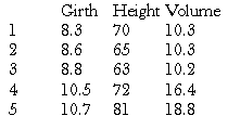
gives us the first 5 rows of these data, and we can now see that the columns represent measurements of girth, height and volume of trees respectively.

Now, if we want to work on the columns of these data, we can use the subscripting technique explained above: for example, trees[,2]gives all of the heights. This is a bit tedious however, and it would be easier if we could refer to the heights more explicitly. We can achieve this by attaching to the trees dataset:

> attach(trees)

Effectively, this makes the contents of trees a directory, and if we type the name of an object, R will look inside this directory to find it. Since Height is the name of one of the columns of trees, R now recognises this object when we type the name. Hence, for example,

> mean(Height)

[1] 76

and

> mean(trees[,2])

[1] 76

are synonymous, while it is easier to remember exactly what calculation is being performed by the first of these expressions. In actual fact, trees is an object called a data frame, essentially a matrix with named columns (though a data frame, unlike a matrix, may also include non-numerical variables, such as character names). Because of this, there is another equivalent syntax to extract, for example, the vector of heights:

> trees$Height

which can also be used without having first attached to the dataset.

Statistical Computation and Simulation

Many of the tedious statistical computations that would once have had to have been done from statistical tables can be easily carried out in R. This can be useful for finding confidence intervals etc. Let’s take as an example the Normal distribution. There are functions in R to evaluate the density function, the distribution function and the quantile function (the inverse distribution function). These functions are, respectively, dnorm, pnorm and qnorm. Unlike with tables, there is no need to standardize the variables first. For example, suppose , then

> dnorm(x,3,2)

will calculate the density function at points contained in the vector x (note, dnorm will assume mean 0 and standard deviation 1 unless these are specified. Note also that the function assumes you will give the standard deviation rather than the variance. As an example

> dnorm(5,3,2)

[1] 0.1209854

evaluates the density of the N(3;4) distribution at x= 5. As a further example

> x<-seq(-5,10,by=.1)

> dnorm(x,3,2)

calculates the density function of the same distribution at intervals of 0.1 over the range [¡5;10].

The functions pnorm and qnorm work in an identical way.

Similar functions exist for other distributions. For example, dt, pt and qt for the t-distribution, though in this case it is necessary to give the degrees of freedom rather than the mean and standard deviation. Other distributions available include the binomial, exponential, Poisson and gamma, though care is needed interpreting the functions for discrete variables.

One further important technique for many statistical applications is the simulation of data from specified probability distributions. R enables simulation from a wide range of distributions, using a syntax similar to the above. For example, to simulate 100 observations from the N(3;4) distribution we write

> rnorm(100,3,2)

Similarly, rt, rpois for simulation from the t and Poisson distributions, etc.