Hypothesis Testing

A hypothesis is a theory about the relationships between variables. Statistical analysis is used to determine if the observed differences between two or more samples are due to random chance or to true differences in the samples.

Basics

A hypothesis is a value judgment, a statement based on an opinion about a population. It is developed to make an inference about that population. Based on experience, a design engineer can make a hypothesis about the performance or qualities of the products she is about to produce, but the validity of that hypothesis must be ascertained to confirm that the products are produced to the customer’s specifications. A test must be conducted to determine if the empirical evidence does support the hypothesis.

Hypothesis testing involves

1. drawing conclusions about a population based on sample data
2. testing claims about a population parameter
3. providing evidence to support an opinion
4. checking for statistical significance

A hypothesis could center around the effect on customer satisfaction if you dramatically improve the time to answer calls from people who are calling for assistance, as well as the amount of time it takes to provide a quality answer right the first time.

There are two categories of hypothesis testing –

1. Descriptive – Descriptive hypotheses concern what you can physically measure about a variable like size, form, etc For example, it could center around your capability to control the wall thickness of a plastic pipe very tightly throughout the entire circumference, for example, and the effect that might have on the weight per foot of pipe.
2. Relational – It involves testing whether the relationship between variables is positive, negative, greater than a given value, or less than a given value. A relational hypothesis could center around the effect on customer satisfaction if you dramatically improve the time to answer calls from people who are calling for assistance, for example, as well as the amount of time it takes to provide a quality answer right the first time.

Hypothesis tests include – the 1-sample hypothesis test for means and the 2-sample hypothesis test for means. In a distribution graph, the 1-sample test has a single mean, which falls to the left of the industry standard. The 2-sample test has two separate mean values. Other types of hypothesis tests include the paired t-test, a test for proportions, a test for variances, and ANOVA, or analysis of variances.

In the paired t-test, for example, you use two sample means to prove or disprove a hypothesis about two different populations. For example, maybe you’re thinking about your test in a customer contact center and if you would find a relationship between the handle-time for the call based on the experience of the technician. You might expect to see a big difference in how long it takes if they have six weeks of training versus six years of experience.

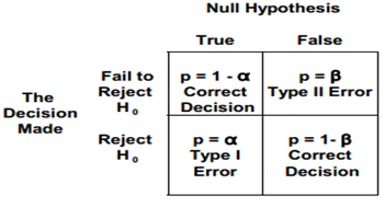
Type I error (False Positive)

It occurs when one rejects the null hypothesis when it is true. The probability of a type I error is the level of significance of the test of hypothesis, and is denoted by *alpha*. An example of a type I error is the notion of producer’s risk. Concluding that something’s bad when it’s actually good is a form of type I error. Other common types of type I errors could be a false alarm, false negative, or an error with the alpha factor or constant that you’re using in your calculations. The alpha or the constant risk is the risk you’re willing to take in rejecting the null hypothesis, when it’s actually true. The common alpha value in most cases is 0.05, giving you a 95% confidence level. What you’re testing for is the possibility of committing a type I error. Usually a one-tailed test of hypothesis is used when one talks about type I error or alpha error.

The alpha significance level signifies that degree or risk of failure that’s acceptable to you. It helps you decide if the null hypothesis can be rejected. Then you have the balance of this and it’s a factor of 1 – α. This is your confidence level acceptance region. This signifies the level of insurance that you expect for the results of the data being studied. It describes the uncertainty associated with the actual sampling method that you’re using.

In a typical distribution curve, a small section of the curve to the left of the peak is the alpha significance level rejection region. The remaining, larger section of the curve is the 1 – α confidence level acceptance region.

Type II error (False Negative)

It occurs when one rejects the alternative hypothesis (fails to reject the null hypothesis) when the alternative hypothesis is true. The probability of a type II error is denoted by *beta*. One cannot evaluate the probability of a type II error when the alternative hypothesis is of the form µ > 180, but often the alternative hypothesis is a competing hypothesis of the form: the mean of the alternative population is 300 with a standard deviation of 30, in which case one can calculate the probability of a type II error.

A type II error relates to beta (β), which is the effect that you’re looking for. You’re looking for the risk associated with the effect of what you’re studying in your dataset.

The most commonly used beta risk is a value of 0.10. An example is, quality assurance risk of failing to find the defective piece during the quality check. It is also called consumer’s risk. Other might also be misdetection, a false positive, or the effect error associated with your data.

Alpha and the beta factors are inversely proportional; reducing the alpha increases the beta, and vice versa.

Decision Rule Determination

The decision rule determines the conditions under which the null hypothesis is rejected or not. The critical value is the dividing point between the area where H0 is rejected and the area where it is assumed to be true.

Decision Making 

Only two decisions are considered, either the null hypothesis is rejected or it is not. The decision to reject a null hypothesis or not depends on the level of significance. This level often varies between 0.01 and 0.10. Even when we fail to reject the null hypothesis, we never say “we accept the null hypothesis” because failing to reject the null hypothesis that was assumed true does not equate proving its validity.

Practical Significance

Practical significance is the amount of difference, change or improvement that will add practical, economic or technical value to an organization.

Statistical Significance

Statistical significance is the magnitude of difference or change required to distinguish between a true difference, change or improvement and one that could have occurred by chance. The larger the sample size, the more likely the observed difference is close to the actual difference.

In testing, you must have statistical significance. It’s the only way to guarantee the strength of your results and support your decisions. In business, though, you also need to have practical significance to back up the decisions you make.

Statistical significance ensures that your results are not by chance; the purpose of your data is to support this theory. Determining statistical significance adds strength to the decisions you make, based on those results.

Practical significance is necessary when the real-world elements, such as cost or time, come into play. Decisions can’t be made solely on statistical significance.

For practical purposes, you should choose values for significance level (α) and power (1 minus β), by carefully considering the consequences of making a type I and type II error. Just as changing the sample size changes the power and significance level of a test, choosing different alpha levels also affects the result of your test.

The traditional value for critical significance, or α, is 0.05, but you can also choose a lower or higher level such as 0.01 or 0.1, depending on what the business situation is. You set the risk level to make the statistical significance more or less sensitive to change.

By setting a more stringent α level, which decreases the probability of making a type I error, you increase the likelihood of making a type II error. When setting the α level, you need to make a good compromise between the likelihood of making type I and type II errors.

To achieve victory in a project, both practical and statistical improvements are required. It is possible to find a difference to be statistically significant but not of practical significance. Because of the limitations of cost, risk, timing, etc., project team cannot implement practical solutions for all statistically significant Xs. Determining practical significance in a Six Sigma project is not the responsibility of the Black Belt alone. Project team need to collaborate with others such as the project sponsor and finance manager to help determine the return on investment (ROI) associated with the project objective.

Practical significance should be considered when setting an α level for statistical significance. You want to find a balance so you don’t find that your results are practically, but not statistically, significant. And just because results are statistically significant doesn’t mean they’re practically significant.

Null Hypothesis

The first step consists in stating the hypothesis. It is denoted by H0, and is read “H sub zero.” The statement will be written as H0: µ = 20%. A null hypothesis assumes no difference exists between or among the parameters being tested and is often the opposite of what is hoped to be proven through the testing. The null hypothesis is typically represented by the symbol Ho. It expresses the status quo, or “what they say.” It assumes that any observed differences are due to chance or random variation. It can also sometimes be expressed with less than or equal to (≤) or greater than or equal to (≥). It also uses the operator equals (=).

Alternate Hypothesis

If the hypothesis is not rejected, exactly 20 percent of the defects will actually be traced to the CPU socket. But if enough evidence is statistically provided that the null hypothesis is untrue, an alternate hypothesis should be assumed to be true. That alternate hypothesis, denoted H1, tells what should be concluded if H0 is rejected. H1 : µ ≠ 20%. An alternate hypothesis assumes that at least one difference exists between or among the parameters being tested. This hypothesis is typically represented by the symbol Ha. It is what you want to test or prove. This assumes that the observed differences are real and not due to chance or random variation. It uses the operators not equal to (≠), greater than (>), and less than (<).

Establishing hypotheses

As you move into establishing your hypothesis, you’ll start with the null hypothesis, represented by H₀. What you’re looking for here is whether the population parameters of interest are equal and there’s really no change or difference. For example, you might have a null hypothesis that humidity would not have an effect on the weight of parts as you’re measuring the weight of parts in a process.

The alternative hypothesis, represented by Hₐ, looks at the population parameters of interest that are not equal, and the difference is real. For example, your hypothesis might be that the greater the level of the experience of your workers would directly correlate to the quality of the output of the work itself or your expectation that men and women would react differently to a change in food ingredients in a product.

A hypothesis test has one of two possible outcomes:

1. reject the null in favor of proving that there is an alternative hypothesis – You need to find out if the result is statistically significant to disprove your hypothesis. For example, does it matter which country people live in with respect to the customer satisfaction level for a given level of service? You’re expecting to find a null, but you could reject it in favor of the alternative hypothesis if you find out that people from different countries have different opinions about the same service level.
2. fail to reject the null hypothesis – In this case, you find insufficient evidence to claim that your null hypothesis was invalid or that an alternative hypothesis is true. For example, when exploring whether ambient humidity in the air affects a plastic product weight over time, you’re expecting to find a yes and you actually do. This would be the alternative hypothesis rejecting it.

The correct way to state the result of the test is to do it in terms of the null hypothesis. For example, state the result as either “we reject the null hypothesis” or “we fail to reject the null hypothesis.”

Estimates

There are two types of estimates – point estimates and interval estimates. Point estimates are used to find a single value to estimate a population parameter, for example the mean.

Point estimates can be classified as the following:

1. When the mean of all possible sample statistic values is equal to the corresponding population parameter, you have an unbiased estimator.
2. When you can make an estimation of a population parameter using more than one possible sample statistic, the statistic with the smaller variance is considered the efficient estimator.

While point estimates offer the best results in certain testing situations, there’s also a downside. When calculating point estimates, sampling error can have an impact on the calculated values. In many cases, point estimates don’t exactly equal the population parameter in a sample. You need another technique to determine how good the estimate is. In that case, you calculate a range, or interval estimates, so that the chances of error are minimized.

A confidence interval allows you to calculate a range within which the population parameter is likely to fall a certain percentage of the time. The range usually spans from a lower confidence limit to an upper confidence limit and the percentage is stated as a level of confidence, which is calculated as 1 minus α.

You can use confidence intervals to check a number of things: the variability of sample statistics, whether a target value falls within the natural variation of a process, and whether two samples originate from the same population.

The correct way to express confidence intervals in words is by stating the confidence level percentage and the interval in which the value is expected to fall with that confidence. Another use of confidence intervals is to examine differences between a population mean and a target value. If the target value does fall within your confidence interval, you know that the sample is from a population with a mean that’s the same as the target value.

Test Statistic

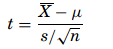
The decision made on whether to reject H0 or fail to reject it depends on the information provided by the sample taken from the population being studied. The objective here is to generate a single number that will be compared to H0 for rejection. That number is called the test statistic. To test the mean µ, the Z formula is used when the sample sizes are greater than 30,

and the t formula is used when the samples are smaller,

Testing for a Population Mean 

When the sample size is greater than 30 and σ is known, the Z formula can be used to test a null hypothesis about the mean. The Z formula is as

Phrasing 

In hypothesis testing, the phrase “to accept” the null hypothesis is not typically used. In statistical terms, the Six Sigma Black Belt can reject the null hypothesis, thus accepting the alternate hypothesis, or fail to reject the null hypothesis. This phrasing is similar to jury’s stating that the defendant is not guilty, not that the defendant is innocent.

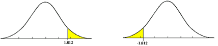
One Tail Test 

In a one-tailed t-test, all the area associated with a is placed in either one tail or the other. Selection of the tail depends upon which direction to bs would be (+ or -) if the results of the experiment came out as expected. The selection of the tail must be made before the experiment is conducted and analyzed.

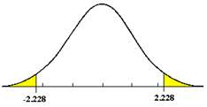
Two Tail Test 

If a null hypothesis is established to test whether a population shift has occurred, in either direction, then a two tail test is required. The allowable a error is generally divided into two equal parts.

A hypothesis test may be one-tailed or two-tailed, as follows:

1. if your alternative hypothesis is “The mean is going to be greater than the hypothesis mean”, you would find a one-tailed test to the right
2. if your hypothesis is “The hypothesis mean is going to be greater than the mean”, you would have a one-tailed test to the left
3. if your alternative hypothesis is “The mean would not be equal”, you would have a two-tailed test with defects on both sides of the data curve

Finding the critical value is about finding that cut-off value for the completed test statistics that defines the statistical significance that you’re seeking in your study. You use the concept of critical value to compute the margin of error and this is derived by multiplying the critical value by the standard deviation of the statistic or by the standard error of the statistic.

The degrees of freedom, or df, is found by taking the number of subjects in your study and subtracting 2. The alpha factors column headers are the various alpha factors you can choose in your study. For example, if you had an alpha factor of 0.5 for a 95% confidence interval and your df is 5, the critical factor identified in a table might be 2.015.

A one-tailed test is used to determine whether your values are greater than a set value – one-tailed to the right – or less than a set value – one-tailed to the left. You use a two-tailed test to determine whether your results come within set boundaries or critical values, or fall below or above your possible results.

Once you’ve reached this part of hypothesis testing, you’ve determined your alpha level. So you need to conclude your hypothesis by using either the critical value method or the p-value method. You find the test statistic using your collected data and a formula depending on which type of test you are conducting – z-test, t-test, F-test, or chi-square. You then find the critical value by using the degree of freedom and significance level (α) with the correct associated table.

The test statistic is derived using the following formula: z = Xbar – µ / (σ / square root of n)

One-tailed test to the right

In a chart that demonstrates a one-tailed test to the right, the 1 – α acceptance region is a large section of the left side of the chart. The rejection region is a small section on the right, which begins at the critical value, based on α.

The alternative hypothesis is that the mean is greater than the hypothesis mean. If the test statistic falls into the rejection region, you would reject the null hypothesis. The acceptance region is the confidence level of a test, of 1 – α or constant factor. If α is 5%, the resulting confidence level would be 95%.

One-tailed test to the left

In a chart that demonstrates a one-tailed test to the left, the 1 – α acceptance region is a large section of the right side of the chart. The rejection region is a small section on the left, which ends at the critical value that’s based on α.

The alternative hypothesis is that the mean is less than the hypothesis mean. If the test statistic is greater than the critical value, it’s outside the rejection area and you would fail to reject the null hypothesis.

Two-tailed test

You use a two-tailed test to test for the actual mean. The majority of tests in real-life situations are of this type. You want to test if that actual mean does not equal the hypothesized mean. For a two-tailed test, you would divide α by 2 since there are two rejection regions that you’re interested in finding, on either side of the tail.

As an example, you want to examine the quantity of chocolate covered peanuts per bag of product that you’re going to ship to your customers. You’re aiming for the average count of 30 to 35 chocolate covered peanuts per bag. If you have too few peanuts per bag, the customers will be unhappy. Conversely, on the right-hand side, if you have more than 35 peanuts, your customer won’t care. They’ll probably like it but that will represent a financial loss for the organization, because you’re consistently putting too much product into the bag.

You want to understand the issues associated with putting too few or too many peanuts in a bag. You want to make sure that your values are going to be consistent inside the acceptance region. If the test statistic is not in either of the rejection regions, you would fail to reject the negative hypothesis.

Hypothesis Test Power

The power of a hypothesis test is measured as 1 – beta (β). The power, or sensitivity, of a statistical test is the probability of it rejecting the null hypothesis when it’s false. You can also think of this as the probability of correctly accepting the alternative hypothesis when it’s true, or the ability of a test to detect a defect.

Determining the power of a test, and minimum and maximum power values, can help you increase the chances of correctly accepting or rejecting a null hypothesis.

Factors that affect the power of a test

Factors that affect the power of a test include – sample size, population differences, variability and alpha (α) level. For example, if you’re looking at equivalency exams testing in education, it’s been shown that the power of testing is influenced by the size of the samples, the amount of variability, and the size of the differences in the populations of students that you might be studying.

1. Sample size – Of all of the factors affecting the power of a test, the sample size is the most important because this is something you can easily control. The power of a test increases with sample size. However, the sample size should be determined very carefully. Samples that are too large could waste time, money, and resources without adding a lot of value. Samples that are too small can lead to inaccurate results.
2. Population differences – The greater the differences between populations, the more likely you’ll be able to detect the differences and therefore the higher the power of a test. Similarly, as population differences get smaller, the power decreases too. This is particularly important when planning a study. You need to make sure that you have large enough samples to avoid type II errors.
3. Variability – Variability and power are inversely proportional. In other words, less variability corresponds to more power. Similarly, more variability corresponds to less power.
4. α level – You can determine the level of the alpha you want for your test, and this is very important. The most common value you would pick is 0.05. You use this to determine the critical value. However, decreasing this value can definitely change the overall results of your test. When you compare your p-value against this value, the higher alpha means that you would have more power. For example, an alpha value of 0.01 results in lower power for a hypothesis test than an alpha value of 0.05.

p-values

A p-value is used to determine statistical significance and to evaluate how well data supports a null hypothesis. It includes the effect size, sample size, and variability of data. A low p-value indicates that the sample data contains enough evidence to reject the null hypothesis for the population.

Consider how alpha (α) and p-values compare. In an example distribution, you have a p-value of 0.2. Given a 95% confidence interval, this value is not in the reject zone. Therefore, you would fail to reject the null hypothesis. In a second distribution with a much lower p-value of 0.02, the confidence interval would actually get smaller and you’d see the p-value showing up in the reject zone. Therefore, you’d reject the null hypothesis.

If the p-value is less than the alpha factor – often the α factor would be at a 95% and the confidence level would be a 0.05 – you would say the test is significant and you can reject the null hypothesis. However, if the p-value is greater than the α value, you would not reject the null hypothesis. A way to remember this is the saying “If p is high, null will fly. If p is low, null will go.”

As an example, you might have sample data about temperature and weight. If there’s a p-value of 0.002 for temperature, it’s likely that the p-value falls in the α rejection region. Therefore, you would reject the null hypothesis around temperature.

If weight has a p-value of 0.423, it’s very likely that you wouldn’t reject that particular null hypothesis.

Sample Size

It has been assumed that the sample size (n) for hypothesis testing has been given and that the critical value of the test statistic will be determined based on the a error that can be tolerated. The sample size (n) needed for hypothesis testing depends on the desired type I (a) and type II (b ) risk, the minimum value to be detected between the population means (m – m0) and the variation in the characteristic being measured (S or s).

The steps for performing hypothesis testing are

1. Define the practical problem. From the Define and Measure phases, we have used tools such as the cause-and-effect diagram, process mapping, matrix diagrams, FMEA and graphical data analysis to identify potential Xs. Now statistical testing is needed to determine significance.
2. Define the practical objective. Define logical categorizations where differences might exist so that meaningful action can be taken. Determine what to prove (i.e., what questions will the hypothesis test answer?)
3. Establish hypotheses to answer the practical objective. The following is an example of hypotheses using a test of means where the mean of each shift is equal against the alternative where they are not equal Null Hypothesis is Ho: μ1st shift= μ2nd shift= μ3rd shift then, alternate hypothesis is Ha: At least one mean is different
4. Select the appropriate statistical test. Based on the data that has been collected and the hypothesis test established to answer the practical objective, refer to the Hypothesis Testing Road Map to select statistical tests. The roadmap is a very important tool to use with each hypothesis test.
5. Define the alpha (α) risk. The Alpha Risk (i.e., Type II Error or Producer’s Risk) is the probability of rejecting the null hypothesis when it is true (i.e., rejecting a good product when i meets the acceptable quality level). Typically, (α) = 0.05 or 5%. This means there is a 95% (1-α) probability it is failing to reject the null hypothesis when it is true (correct decision).
6. Define the beta (β) risk. The Beta Risk (i.e., Type II Error or Consumer’s Risk) is the probability of failing to reject the null hypothesis when there is significant difference (i.e., a product is passed on as meeting the acceptable quality level when in fact the product is bad). Typically, (β) = 0.10 or 10%.
7. Establish delta (δ). Delta (δ) is the practical significant difference detected in the hypothesis test between

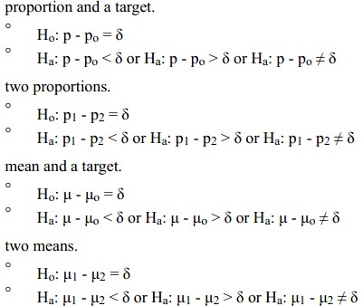
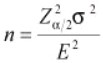
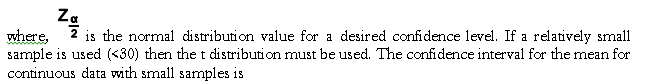
1. Determine the sample size (n). Sample size depends on the statistical test, type of data and alpha and beta risks. There are statistical software packages to calculate sample size. It is also possible to manually calculate sample sizes using a sample size table. Using the formula below, where the data is continuous and Z = 1.96 at a confidence level of 95% (α/2 = 0.025 Two Tail Test), σ2 is the standard deviation, and E is the margin of error (the range of values around the estimate that probably contains the true value).

1. Conduct the statistical tests. Use the Hypothesis Test blueprint to lead in the right direction for the type of data collected.
2. Collect the data. Data collection is based on the sampling plan and method.
3. Develop statistical conclusions. The p–value is the smallest level of significance that would lead to rejection of the null hypothesis (Ho). Usually, if α = 0.05 and the p-value ≤ 0.05, then reject the null hypothesis and conclude that there is a significant difference. But, if α = 0.05 and the p-value > 0.05, then fail to reject the null hypothesis and conclude that there is not a significant difference.
4. Determine the practical conclusions. Restate the practical conclusion to reflect the impact in terms of cost, return on investment, technical, etc. Remember, statistical significance does not imply practical significance.

Tests for means, variances and proportions

Confidence Intervals for the Mean 

The confidence interval for the mean for continuous data with large samples is

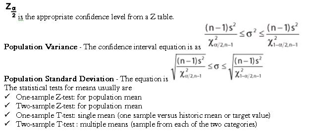
Confidence Intervals for Variation 

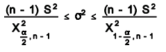
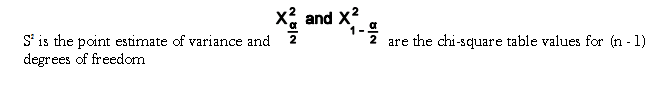
The confidence intervals for variance is based on the Chi-Square distribution. The formula is

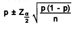
Confidence Intervals for Proportion

For large sample sizes, with n(p) and n(1-p) greater than or equal to 4 or 5, the normal distribution can be used to calculate a confidence interval for proportion. The following formula is used

One-Sample Z-Test for Population Mean

The One-sample Z-test for population mean is used when a large sample (n≥ 30) is taken from a population and we want to compare the mean of the population to some claimed value. This test assumes the population standard deviation is known or can be reasonably estimated by the sample standard deviation and uses the Z distribution. Null hypothesis is Ho: μ = μ0 where, μ0 is the claim value compared to the sample.

Two-Sample Z-Test for Population Mean

The Two-sample Z-test for population mean is used after taking 2 large samples (n≥30) from 2 different populations in order to compare them. This test uses the Z-table and assumes knowing the population standard deviation, or estimated by using the sample standard deviation. Null hypothesis is Ho: μ1= μ2

One-Sample T-test 

The One-sample T-test is used when a small sample (n< 30) is taken from a population and to compare the mean of the population to some claimed value. This test assumes the population standard deviation is unknown and uses the t distribution. The null hypothesis is Ho: μ = μ0 where μ0 is the claim value compared to the sample. The test statistic is

where x is the sample mean, s is the sample standard deviation and n is the sample size.

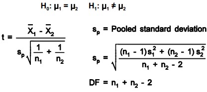
Two-Sample T-test

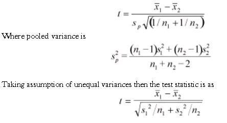
The Two-sample T-test is used when two small samples (n< 30) are taken from two different populations and compared. There are two forms of this test: assumption of equal variances and assumption of unequal variances. The null hypothesis is Ho: µ1= µ2. The Test Statistic with assumption of equal variances is

One-sample Tests for Means

When considering which hypothesis test to use, you must first consider the purpose of your study and then the population parameter to be tested, be it means, proportions, or variances. The hypothesis test for means helps determine if the differences between either a sample mean and a hypothesized value, or between two or more sample means, are due to natural variability or real differences.

Hypothesis tests for means allow you to accomplish two things: evaluate claims about the performance or characteristics of a process, product, or service, and compare performance before and after an improvement effort.

The three types of hypothesis tests for means include the following:

1. A one-sample test for means, also known as a one-population test for means, compares the mean of a sample from a population against a hypothesized, or specified, value. This specified value can be an expected or desired value, a historical value, an industry benchmark, or a customer specification.
2. A two-sample test for means, also known as a two-population test for means, compares the means of two samples. The two samples may or may not be from the same population.
3. You can compare the means of two or more samples by using analysis of variance (ANOVA).

One-sample and two-sample tests for means can be of two types:

1. When the variance of the larger population is unknown and the sample size is less than 30, a t-test is used to calculate a test statistic. You will then use a t-distribution table and the degrees of freedom to interpret your results.
2. When the variance of the larger population is known, a z-test is used. Even if population variance is not known, you’ll recall that the central limit theorem allows you to estimate population parameters using sample statistics when sample size is sufficiently large. Therefore, z-tests are typically used when n is greater than or equal to 30. With this test, you calculate a z-statistic and use a z-table to make your conclusions.

One-sample and two-sample tests for means are parametric tests; therefore, it’s a requirement that the data being tested is normally distributed.

To begin the process of hypothesis testing, you need a null hypothesis to be tested. Then you can formulate an analysis plan, analyze sample data according to the plan, reject or fail to reject the null hypothesis, and make a decision based on the test. Usually, a five-step procedure is adopted for testing a hypothesis to determine if it is to be rejected, or not, beyond a reasonable doubt

1. Define the business problem – specifically what the test will compare or validate.
2. Establish the hypotheses. Once you know the problem, you can define the two possible answers by the null and alternative hypotheses. The null hypothesis (H0) is traditionally the hypothesis of no change. It assumes that any difference between samples results from random variation or noise. The alternative hypothesis (Ha) is the hypothesis of change. It assumes that observed difference is real.
3. Determine the test parameters. After establishing your hypotheses, you decide how to conduct your hypothesis test. There are a number of considerations, including selecting the appropriate statistical test, identifying key test considerations such as degrees of freedom and alpha value, conducting sampling, and doing normality checks.
4. Calculate the test statistic, which indicates whether your sample data is consistent with, less than, or greater than the population mean. You’ll use the appropriate test for means formula and your sample data to calculate the test statistic.
5. Interpret the results. Once you find the critical value or the p-value to which you compare your test statistic or your alpha value, you can determine whether to reject or fail to reject the null hypothesis. If the test statistic is higher than the critical value, you reject the null hypothesis. If the test statistic is lower than the critical value, it means that your finding is not significant and you fail to reject the null hypothesis.

Evaluating the results in practical terms is important during the interpretation step. You need to ensure that your results have practical significance, as well as statistical significance, before implementing any process changes.

It’s important to note that in real-life Six Sigma situations, statistical modeling and calculations are much more complex and are done using software. You may find a slight numerical difference between the test statistics, p-values, or critical values calculated using software versus those calculated manually. This difference is usually caused by rounding and is not usually significant enough to change the final result.

Hypothesis testing statistically validates your claim about a population using sample data. The three types of hypothesis tests are a one-sample test for means, a two-sample test for means, and a multiple-sample test for means.

One-sample and two-sample tests for means can one of two types – a t-test or a z-test. You choose the appropriate formula based on the size of the sample, or whether the population variance is known. A known variance or a large sample size calls for a z-test, while an unknown variance and a small sample size calls for a t-test. One-sample tests compare the mean of one population to a specified value, such as an industry benchmark, historical value, or customer specification. A five-step process is adopted for testing a hypothesis – define the business problem, establish the null and alternative hypotheses, determine test parameters, calculate the test statistic, and interpret the results.

Two-sample Tests for Means

A one-sample test for means compares the mean of a sample from a population against a hypothesized, or specified, value. This specified value can be an expected or desired value, a historical value, an industry benchmark, or a customer specification.

But a two-sample test for means compares two means, not necessarily from the same population, to determine whether or not there are significant differences between them. The main difference between one-sample and two-sample tests for means is the factors that are being compared.

Like one-sample hypothesis tests for means, two-sample tests can make use of z-tests or t-tests, depending on the available data about population variance and sample size. Likewise, depending on the method most preferred by you or your organization, the tests may employ either the critical value or p-value method. As with the one-sample test for means, you can follow the same five hypothesis-testing steps to complete a two-sample test

1. define the business problem
2. establish the hypotheses
3. determine the test parameters
4. calculate the test statistic
5. interpret the results

When working with a two-sample test for means, you will need to consider the following elements

1. With a two-sample test for means, the hypotheses typically use the equal to symbol for the null hypothesis and can use the not equal to, less than, or greater than symbols for the alternative hypothesis.
2. With a two-sample test for means, there are two conditions to examine and two possible formulas to choose from. So it’s important to ensure you’re applying the right formula – pooled or non-pooled.
3. You must also consider the distribution. You generally assume when performing a two-sample test for means that the two samples are independent and random and from normally distributed populations. Also, in most cases, you’ll assume the two samples have unequal variances.

As with a one-sample test for means, you can use a flowchart to help select the correct formula. And like the one-sample test, when the population variance is known or n is greater than or equal to 30, the z-test is used.

However, when n is less than 30 and you don’t know the variance of the population, the t-test is further broken down into two formulas – pooled and non-pooled. You use the two-sample test for means pooled formula when population variances are unknown but considered to be equal.

You use the non-pooled formula when population variances are unknown and considered to be unequal. There is also a special formula for determining the degrees of freedom for a non-pooled two-sample t-test.

A two-sample test for means compares two means to determine whether or not there are significant differences between them. As with the one-sample test for means, you can follow the five hypothesis-testing steps to complete a two-sample test. The steps are to define the business problem, establish the hypotheses, determine test parameters, calculate the test statistic, and finally, interpret the results.

If the sample size is large, or population variances are known, you use a z-test. And when population variances are unknown and sample size is less than 30, you use a t-test. This is further broken down into two formulas – pooled and non-pooled.

The two-sample test for means pooled formula is used when population variances are considered to be equal. The non-pooled formula is used when population variances are considered to be unequal.

Tests for Variances

When performing hypothesis tests, the population’s variance or standard deviation is often of greater significance than the population mean. It can be crucial to confirm that the observed variance of a population is actually at the value that you expect or require.

To compare the variance in a single population with a specified value, you use a one-sample test for variance. All tests for variance follow the usual five-step process for hypothesis testing.

What are the unique features of one-sample tests for variances? You need to consider four key areas: test statistic, critical value, degrees of freedom, and data.

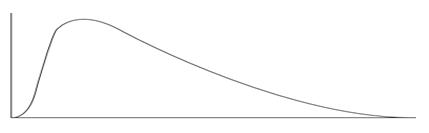
The chi-square distribution, used in one-sample variance tests, is not symmetric but skewed to the right. It is highly skewed for small degrees of freedom, but becomes more and more symmetric as the degrees of freedom increase. It must also be assumed that the data is continuous, independent, and randomly sampled.

The one-sample test for variance can benefit an organization in two ways:

1. it can let a team know that a process’s variation is within an expected range and therefore not in need of improvement
2. it can let the team know that a process’s variation is not within a required range, therefore targeting the process for improvement

Two-sample tests for variance

If you wish to determine which of two samples exhibits the largest variance, you use a two-sample test for variance. The population samples for this test may come from two different processes, or from the same process at two different times – for example, before and after an improvement initiative.

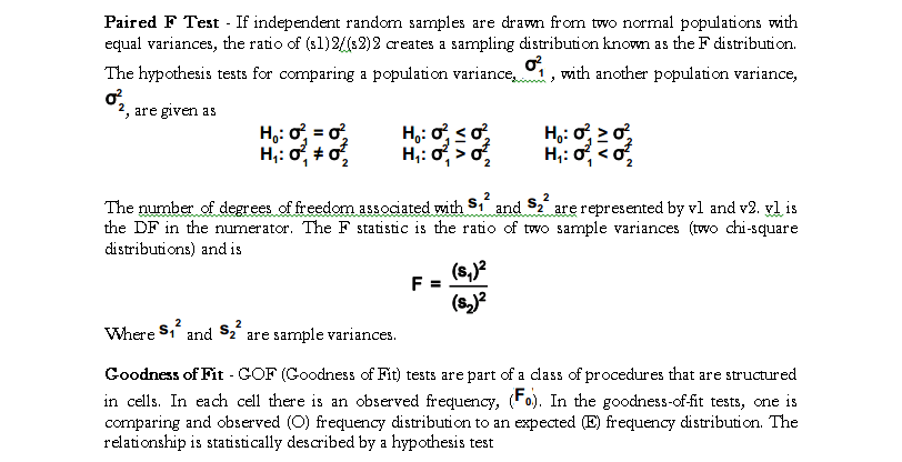
In a two-sample test for variance, you use the F-test to compare the variances between two populations. The F distribution is used to plot the ratio of two variances. For the F-test to be used as a test statistic, the data must be normally distributed, as well as independent, randomly sampled, and continuous.

To determine significance, you can compare the F-statistic to the critical value in a table, or you can calculate the p-value, which is typically done using statistical software.

Paired-comparison tests

They are powerful ways to compare data sets by determining if the means of the paired samples are equal. Making both measurements on each unit in a sample allows testing on the paired differences. An example of a paired comparison is two different types of hardness tests conducted on the same sample.

Once paired, a test of significance attempts to determine if the observed difference indicates whether the characteristics of the two groups are the same or different. A paired comparison experiment is an effective way to reduce the natural variability that exists among subjects and tests the null hypothesis that the average of the differences between a series of paired observations is zero.

Paired t Test

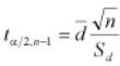
In paired t-test for two population means each paired sample consists of a member of one population and that member’s corresponding member in the other population. It tests the difference between 2 sample means. Data is taken in pairs with the difference calculated for each pair. H0: m1 = m2 and H1: m1 ≠ m2 and DF = n – 1. A paired t test is always a two tail test where = average of differences of pairs of data.

The paired method (dependent samples), compared to treating the data as two independent samples, will often show a more significant difference because the standard deviation of the d’s (Sd) includes no sample to sample variation. This comparatively more frequent significance occurs despite the fact that “n – 1” represents fewer degrees of freedom than “n1 + n2 -2.” The paired t test is a more sensitive test than the comparison of two independent samples.

The steps are

1. Establish the hypotheses – The established hypothesis test is a two-tail test when Ha is a statement of does not equal (≠), left-tail test when Ha has the < sign and right-tail test when Ha has the > sign
2. Calculate the test statistic which is

1. Ho: Random variable is distributed as a specific distribution with given parameters.
2. Ha: Random variable does not have the specific distribution with given parameters.

The formula for calculating the chi-square test statistic for this one-tail test is

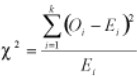
We can calculate the expected or theoretical frequency, (F_e). Chi Square ( X²) is then summed across all cells as

Single-factor analysis of variance (ANOVA)

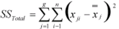
Sometimes it is essential to compare three or more population means at once with the assumptions as the variance is the same for all factor treatments or levels, the individual measurements within each treatment are normally distributed and the error term is considered a normally and independently distributed random effect. With analysis of variance, the variations in response measurement are partitioned into components that reflect the effects of one or more independent variables. The variability of a set of measurements is proportional to the sum of squares of deviations used to calculate the variance .

Analysis of variance partitions the sum of squares of deviations of individual measurements from the grand mean (called the total sum of squares) into parts: the sum of squares of treatment means plus a remainder which is termed the experimental or random error.

ANOVA is a technique to determine if there are statistically significant differences among group means by analyzing group variances. An ANOVA is an analysis technique that evaluates the importance of several factors of a set of data by subdividing the variation into component parts. ANOVA tests to determine if the means are different, not which of the means are different Ho: μ1= μ2= μ3 and Ha: At least one of the group means is different from the others.

ANOVA extends the Two-sample t-test for testing the equality of two population means to a more general null hypothesis of comparing the equality of more than two means, versus them not all being equal.

One-Way ANOVA

Terms used in ANOVA

1. Degrees of Freedom (df) – The number of independent conclusions that can be drawn from the data.
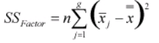
2. SSFactor – It measures the variation of each group mean to the overall mean across all groups.
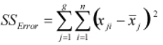
3. SSError – It measures the variation of each observation within each factor level to the mean of the level.
4. Mean Square Error (MSE) – It is SSError/ df and is also the variance.
5. F-test statistic – The ratio of the variance between treatments to the variance within treatments = MS/MSE. If F is near 1, then the treatment means are no different (p-value is large).
6. P-value – It is the smallest level of significance that would lead to rejection of the null hypothesis (Ho). If α = 0.05 and the p-value ≤ 0.05, then reject the null hypothesis and conclude that there is a significant difference and if α = 0.05 and the p-value > 0.05, then fail to reject the null hypothesis and conclude that there is not a significant difference.

One-way ANOVA is used to determine whether data from three or more populations formed by treatment options from a single factor designed experiment indicate the population means are different. The assumptions in using One-way ANOVA is all samples are random samples from their respective populations and are independent, distributions of outputs for all treatment levels follow the normal distribution and equal or homogeneity of variances.

Steps for computing one-way ANOVA are

1. Establish the hypotheses. Ho: μ1= μ2= μ3 and Ha: At least one of the group means is different from the others.

Calculate the test statistic. Calculate the average of each call center (group) and the average of the samples.

1. Calculate SSFactor as
2. Calculate SSError as
3. Calculate SSTotal as
4. Calculate the ANOVA table with degrees of freedom (df) is calculated for the group, error and total sum of squares.
5. Determine the critical value. Fcritical is taken from the F distribution table.
6. Draw the statistical conclusion. If Fcalc< Fcritical fail to reject the null hypothesis and if Fcalc > Fcritical, reject the null hypothesis.

Hypothesis tests, such as z-tests and t-tests, are useful for testing the values of a single population mean or the difference between two means. But, sometimes it’s necessary to compare three or more population means simultaneously.

ANOVA, or analysis of variance, is a special application of the two-sample t-test for means that allows you to compare the means of three or more populations. So, to perform a hypothesis test to find out whether three levels of temperature significantly affect the moisture content of a product, you use ANOVA instead of the two-sample t-test. ANOVA can be applied to any number of datasets recorded from any process using statistical software packages. It uses samples from each dataset to test the null hypothesis that all population means are equal.

In one-way ANOVA, or single-factor ANOVA, the total variation in the data consists of two parts:

1. the variation among treatment means
2. the variation within treatments, or experimental error

In two-way ANOVA, or two-factor ANOVA, there are three components of variance: factor A treatments, factor B treatments, and experimental error. When using ANOVA, you need to consider three key concepts: factor, level, and response. A factor is a categorical variable, which means that it classifies people, objects, or events. A level is a group within the factor. The response is the variable you are interested in testing. It’s important to distinguish between within-group variation and between-group variation.

Within-group variation, or experimental error, occurs when there is variability between measurements within a single group or factor level. In one-way ANOVA, this is always assumed to be due to experimental error.

Between-group variation occurs where there is variability in measurements between all groups. ANOVA compares between-group variation to within-group variation to determine whether there are significant differences in means between groups.

Performing one-way ANOVA

The two variations are compared using the F-statistic. The F-statistic uses the two variance values in ANOVA to calculate a ratio of variance. The numerator, between-group variance, is the sum of factor-related variance between treatment groups. The denominator, within-group variance, is the sum of error-related variance within treatment groups.

Calculating the F-statistic – that is, the ratio of between-group variation to within-group variation – will allow you to determine whether the between-treatment variation is a large enough multiple of the within-treatment variation to be statistically significant.

The first step in conducting the hypothesis test is to define the business problem. As you define the problem, you must also verify that the three assumptions for ANOVA are met. You can verify the three assumptions using residuals analysis. A residual is the difference between the observed value and the fitted value or the group mean. Residuals are estimates of the error in ANOVA.

The second step of the process is to establish the hypotheses. For one-way ANOVA, the null hypothesis is typically that the mean for each level is equal to the mean for the other levels. The third step is to determine the test parameters. This means setting the alpha risk value and calculating degrees of freedom for each source of variation – that is, for the numerator and denominator of the F-statistic.

The fourth step is to calculate the test statistic. There are several components used in ANOVA to calculate the test statistic, and these will be familiar to you from your Green Belt studies. However, there are four intermediate values used in calculating the test statistic that may be new to you

1. C – C is the correction factor and is calculated using the value T, the grand total of readings, and N, the total number of readings.
2. T – T or Ti is the grand total of readings and is used in the calculation of C.
3. SSFactor – SSFactor is the sum of squares between treatments. You can calculate SSFactor using a more cumbersome summation formula, but this simpler short-cut formula makes use of the easily calculated T and C values.
4. SSTotal – SSTotal is the total sum of squares, and is calculated using this formula. An easier way to calculate it is by adding together SSFactor and SSError. While you can calculate SSTotal using a summation formula, this simpler formula makes use of the easily calculated C value.

You calculate the values for the test statistic using an ANOVA table. The table consists of columns for sources of variation, sums of squares, degrees of freedom, and mean squares for both between-group and within-group variations.

Once the ANOVA table is filled in, the next step is to interpret the results. As with all hypothesis tests, such as the t-test, you have two choices for validating the results: the critical value method, which involves looking up the critical value on an F table; or the p-value method, which involves calculating the p-value for the F-statistic and comparing it to the alpha risk value. Most statistical packages use the p-value method. You can also determine this value using a table.

While ANOVA helps to determine whether the population means for all levels are equal, you can also use some advanced tools to identify which means are different from the rest.

Chi Square

Usually the objective of the project team is not to find the mean of a population but rather to determine the level of variation of the output like to know how much variation the production process exhibits about the target to see what adjustments are needed to reach a defect-free process.

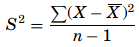
If the means of all possible samples are obtained and organized we can derive the sampling distribution of the means similarly for variances, the sampling distribution of the variances can be known but, the distribution of the means follows a normal distribution when the population is normally distributed or when the samples are greater than 30, the distribution of the variance follows a Chi square (χ2) distribution. As the sample variance is computed as

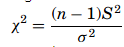
Then the χ2 formula for single variance is given as

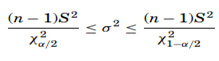
The shape of the χ2 distribution resembles the normal curve but it is not symmetrical, and its shape depends on the degrees of freedom. The χ2 formula can be rearranged to find σ2. The value σ2 with a degree of freedom of n−1, will be within the interval

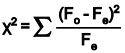
The chi-square test compares the observed values to the expected values to determine if they are statistically different when the data being analyzed do not satisfy the t-test assumptions. The chi-square goodness-of-fit test is a non-parametric test which compares the expected frequencies to the actual or observed frequencies. The formula for the test is

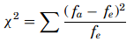
with fe as the expected frequency and fa as the actual frequency. The degree of freedom will be given as df= k − 1. Chi-square cannot be negative because it is the square of a number. If it is equal to zero, all the compared categories would be identical, therefore chi-square is a one-tailed distribution. The null and alternate hypotheses will be df= k − 1.

Chi-square cannot be negative because it is the square of a number. If it is equal to zero, all the compared categories would be identical, therefore chi-square is a one-tailed distribution. The null and alternate hypotheses will be H0: The distribution of quality of the products after the parts were changed is the same as before the parts were changed. H1: The distribution of the quality of the products after the parts were changed is different than it was before they were changed.

Comparing a population’s variance to a standard value involves calculating the chi-square test statistic. Other problems requiring the chi-square test statistic include determining whether one variable is dependent upon another, or comparing observed and expected frequencies where the variance is unknown. The following are hypothesis testing situations regarding different uses of the chi-square test statistic in Six Sigma

1. comparing variance to a standard value
2. determining whether one variable is dependent upon another
3. comparing observed and expected frequencies where variance is unknown

Goodness-of-fit tests employ the chi-square test statistic and share some other similarities with contingency tables, which also compare observed and expected frequencies. But contingency tables and goodness-of-fit tests differ in their goals, hypotheses, and interpretations.

The goal of goodness-of-fit tests is to test assumptions about the distributions that fit the process data. Essentially, a goodness-of-fit test asks if the observed frequencies (O) are the same or different from the historical, expected, or theoretical frequencies (E). If there’s a difference between them, this suggests that the distribution model expressed by the expected frequencies does not fit the data.

Goodness-of-fit tests can be structured in table cells. In one column of the table, each cell contains an observed frequency – Fo or O. Depending on the nature of the problem, the theoretical or expected frequency – Fe or E – is already known or can be calculated. You then use the chi-square formula to calculate and sum the chi-square statistic across all cells. Observed frequencies are the frequencies actually obtained from the sample data in the table. Expected frequencies are the frequencies you would expect in each cell of the table, if you knew only the row and column totals, and if you assumed that the variables being compared were independent.