This phase uses the tools and methods for determining and verifying the sources of variation (input variables – x) as identified by well-designed experiments who input variables to demonstrate the Y = f(x) relationship, where Y is a dependent variable and a function of x. Using a design of experiments (DOE) approach produces information on the relationships between factors so that project team improves the process.
It is a method of varying a number of input factors simultaneously in a planned manner, so that their individual and combined effects on the output can be identified. It develops well-designed efforts to identify which process changes yield the best possible results for sustained improvement as mostly experiments address only one factor at a time, the Design of Experiments (DOE) method focuses on multiple factors at one time. It provides the data that illustrates the significance to the output of input variables acting alone or interacting with one another. Various DOE advantages include evaluation of multiple factors simultaneously, controlling of input factors to make the output insensitive to noise factors, experiments highlight important factors, and there is confidence in the conclusions drawn. the factors can easily be set at the optimum levels and quality and reliability can be improved without cost increase or cost savings can be achieved.
Terminology
Basic DOE terms are
- Factor – A predictor variable that is varied with the intent of assessing its effect on a response variable. Most often referred to as an “input variable.”
- Factor Level – It is a specific setting for a factor. In DOE, levels are frequently set as high and low for each factor. A potential setting, value or assignment of a factor of the value of the predictor variable like, if the factor is time, then the low level may be 10 minutes and the high level may be 30 minutes.
- Response variable – A variable representing the outcome of an experiment. The response is often referred to as the output or dependent variable.
- Treatment – The specific setting of factor levels for an experimental unit. For example, a level of temperature at 65° C and a level of time at 45 minutes describe a treatment as it relates to an output of yield.
- Experimental error – An error from an experiment reveals variation in the outcome of identical tests. The variation in the response variable beyond that accounted for by the factors, blocks, or other assignable sources while conducting an experiment.
- Experimental run – A single performance of an experiment for a specific set of treatment conditions.
- Experimental unit – The smallest entity receiving a particular treatment, subsequently yielding a value of the response variable.
- Predictor Variable – A variable that can contribute to the explanation of the outcome of an experiment. Also known as an independent variable.
- Repeated Measures – The measurement of a response variable more than once under similar conditions. Repeated measures allow one to determine the inherent variability in the measurement system. Repeated measures are known as “duplication” or ‘repetition.”
- Replicate – A single repetition of the experiment.
- Replication – Performance of an experiment more than once for a given set of predictor variables. Each of the repetitions of the experiment is called a “replicate.” Replication differs from repeated measures in that it is a repeat of the entire experiment for a given set of predictor variables, not just repeat of measurements of the same experiment.
- Replication increases the precision of the estimates of the effects in an experiment. Replication is more effective when all elements contributing to the experimental error are included. In some cases replication may be limited to repeated measures under essentially the same conditions. In other cases, replication may be deliberately different, though similar, in order to make the results more general.
- Repetition – When an experiment is conducted more than once, repetition describes this event when the factors are not reset. Subsequent test trials are run again but not necessarily under the same conditions.
- Blocking – When structuring fractional factorial experimental test trials, blocking is used to account for variables that the experimenter wishes to avoid. A block may be a dummy factor which doesn’t interact with the real factors.
- Box-Behnken – When full second-order polynomial models are to be used in response surface studies of three or more factors, Box- Behnken designs are often very efficient. They are highly fractional, three-level factorial designs.
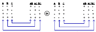
- Confounded – When the effects of two factors are not separable. As in the image below
- Correlation Coefficient (r) – A number between -1 and 1 that indicates the degree of linear relationship between two sets of numbers. Zero (0) indicates no linear relationship.
- Covariates – Things which change during an experiment which had not been planned to change, such as temperature or humidity. Randomize the test order to alleviate this problem. Record the value of the covariate for possible use in regression analysis.
- Degrees of Freedom – The term used is DOF, DF, df or v. The number of measurements that are independently available for estimating a population parameter.
- EVOP – It stands for evolutionary operation, a term that describes the way sequential experimental designs can be made to adapt to system behavior by learning from present results and predicting future treatments for better response.
- First-order – It refers to the power to which a factor appears in a model. If “X1” represents a factor and “B” is its factor effect, then the model Y = B0 + B1X1 + B2X2 + ,is first-order in both X1 and X2.
- Fractional – An adjective that means fewer experiments than the full design.
- Full Factorial – It describes experimental designs which contain all combinations of all levels of all factors. No possible treatment combinations are omitted.
- Interaction – It occurs when the effect of one input factor on the output depends upon the level of another input factor.
- Level – It is a given factor or a specific setting of an input factor like three levels of a heat treatment may be 100°C, 120°C and 150°C.
- Main Effect- An estimate of the effect of a factor independent of any other factors.
- Mixture Experiments – They are experiments in which the variables are expressed as proportions of the whole and sum to 1.0.
- Nested Experiments – An experimental design in which all trials are not fully randomized.
- Optimization – It involves finding the treatment combinations that gives the most desired response. Optimization can be maximization or minimization
- Orthogonal – It is a design is orthogonal if the main and interaction effects in a given design can be estimated without confounding the other main effects or interactions.
- Paired Comparison – The basis of a technique for treating data so as to ignore sample-to-sample variability and focus more clearly on variability caused by a specific factor effect. Only differences in response for each sample are tested because sample-to-sample differences are irrelevant.
- Fixed Effects Model – If the treatment levels are specifically chosen by the experimenter, then conclusions reached will only apply to those levels.
- Random Effects Model – If the treatment levels are randomly chosen from a population of many possible treatment levels, then conclusions reached can be extended to all treatment levels in the population.
- Residual Error () or (E) – The difference between the observed and the predicted value for that result, based on an empirically determined model. It can be variation in outcomes of virtually identical test conditions.
- Residuals – The difference between experimental responses and predicted model values.
- Resolution – A fractional factorial design in which no main effects are confounded with each other but the main effects and two factor interaction effects are confounded.
- Response Surface Methodology (RSM) – The graph of a system response plotted against system factors. RSM employs experimental design to discover the “shape” of the response surface and uses geometric concepts to take advantage of the relationships.
Experiments can be designed to meet a wide variety of experimental objectives as
- Fixed-effects model – An experimental model where all possible factor levels are studied. For example, if there are three different materials, all three are included in the experiment.
- Random-effects model – An experimental model where the levels of factors evaluated by the experiment represent a sample of all possible levels. For example, if we have three different materials but only use two materials in the experiment.
- Mixed model – An experimental model with both fixed and random effects.
- Completely randomized design – An experimental plan where the order in which the experiment is performed is completely random.
The steps for conducting DOE are
- Gain complete knowledge of inputs and outputs with a process flow diagram or process map.
- Finalize the output measure usually variable measure is taken and attribute measures avoided with stable and repeatable measurement system.
- Develop design matrix for the factors under investigation showing all possible combinations of high and low levels for each input factor.
- Obtain extreme high and low levels for every input to investigate.
- Enter the factors and levels for the experiment into the design matrix.
- Perform each experiment and record the results.
- Compute the effect of a factor by averaging the data collected at the low level and subtracting it from the average of the data collected at the high level.
ANOVA is a basic step in the DOE that is a formidable tool for decision-making based on data analysis. The types of ANOVA that are more commonly used are
- The completely randomized experimental design, or one-way ANOVA. One-way ANOVA compares several (usually more than two) samples’ means to determine if there is a significant difference between them.
- The factorial design, or two-way ANOVA, which takes into account the effect of noise factors.
Design Guidelines for DOE are as
| Number of Factors | Comparative Objective | Screening Objective | Response Surface Objective |
| 1 | 1-factor completely randomized design | _ | _ |
| 2-4 | Randomized block design | Full or fractional factorial | Central composite or Box-Behnken |
| 5 or more | Randomized block design | Fractional factorial or Plackett-Burman | Screen first to reduce number of factors |
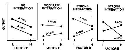
Main Effects
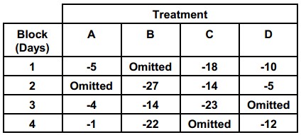
Randomized Block Plans – When each homogeneous group in the experiment contains exactly one measurement on every treatment, the experimental plan is called a randomized block plan. For example, an experimental scheme may take several days to complete. If we expect some biasing differences among days, we might plan to measure each item on each day, or to conduct one test per day on each item. A day would then represent a block. A randomized Incomplete block (tension response) design is shown below.
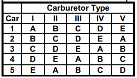
Latin Square Designs – A Latin square plan is useful to allow for two sources of non-homogeneity in the conditions affecting test results. A third variable, the experimental treatment, is then applied to the source variables in a balanced fashion. A Latin square design is essentially a fractional factorial experiment, restricted by two conditions
- The number of rows, columns and treatments must be the same.
- There should be no expected interactions between row and column factors.
For example, 5 automobiles, 5 carburetors are used to evaluate gas mileage by five drivers in the 5 x 5 Latin square
Full factorial experiments
A full factorial is an experimental design which contains all levels of all factors. No possible treatments are omitted. A fractional factorial is a balanced experimental design which contains fewer than all combinations of all levels of all factors. Listed below are full and half fractional factorial designs for 3 factors at two levels
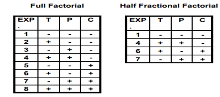
The half fractional factorial also requires an equal number of plus and minus signs in each column.
Taguchi Designs – The Taguchi philosophy emphasizes two tenets of reducing the variation of a product or process which reduces the loss to society and using a proper development strategy to intentionally reduce variation.
Orthogonal Arrays Degrees of Freedom – Let df = Degrees of Freedom, k = number of factor levels then for factor A, dfA = kA – 1 and for factor B, dfB = kB – 1. For A x B interaction, dfAB = dfA x dfB. dfmin= ∑df all factors + ∑df all interactions of interest.
The simplest orthogonal array (OA) is an L4 (four trial runs). Factors A and B can be assigned to any two of the three columns. The remaining column is the interaction column. The effects of factors A, B, AxB are determined for each column. Then calculate SST, SSA, SSB, SSAXB and SSe. A standard ANOVA table can now be set up to determine factor significance at a selected alpha value.
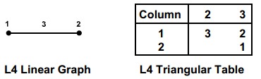
If the two factors are assigned to columns 1 and 2, the interaction will be in column 3. The L4 triangular Table shows that if the two factors are put in columns 1 and 3, the other point of the triangle for the interaction is in column 2.
Design resolution is the degree of confounding in two-level fractional screening designs. That is, the degree to which factors is entangled so that one cannot separate their effects. Resolution II designs will have some main effects confounded with some other main effects. Resolution III designs do not confound main effects with each other, but do confound main effects with two-factor interactions. Resolution IV designs do not confound main effects and two-factor interactions, but do confound two-factor interactions with other two-factor interactions. Resolution V designs do not confound main effects and three-factor interactions, but do confound two-factor interactions with higher-order interactions.
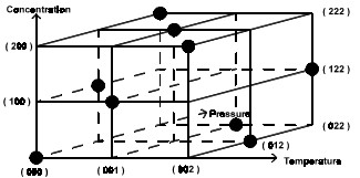
A Three Factor, Three Level Experiment – Often a three factor experiment is required after screening a larger number of variables. These experiments may be full or fractional factorial. Shown below is a 1/3 fractional factorial design. Generally the (-) and (+) levels in two level designs are expressed as 0 and 1 in most design catalogues. Three level designs are often represented as 0, 1 and 2.
The Factorial Design with Two Factors – It tests several treatments simultaneously with the level of very treatment is tested for all treatments. For example the heat generated by a generator depends on its RPM and on the time it is operating. Samples taken while two generators are running for four hours are summarized in table below.
| Hours | 500RPM | 550RPM | 600RPM |
| 1 | 65 | 80 | 84 |
| 65 | 81 | 85 | |
| 2 | 75 | 83 | 85 |
| 80 | 85 | 86 | |
| 3 | 80 | 86 | 90 |
| 85 | 87 | 90 | |
| 4 | 85 | 89 | 92 |
| 88 | 90 | 92 |
With the two-way ANOVA, all the RPMs for every time-frame are observed as well as the timeframes (hours) for every RPM. The row effects and the column effects are called the main effects, and the combined effects of the rows and columns is called the interaction effect.
In this example, a table’s cell is the intersection between an RPM (column) and a length of time (row) and has two observations. Cell 1 is comprised of observations (65, 65). So we have three cells per row and four rows, which make a total of 12 cells. As the two-way ANOVA is also a hypothesis test but with three hypotheses
- The first hypothesis will stipulate that there is no difference between the means of the RPM treatments. H0: µr 1 = µr 2 = µr 3 where µ1, µ2, and µ3 are the means of the RPM treatments.
- The second hypothesis will stipulate that the number of hours that the generators operate does not make any difference on the heat. H0: µh1 = µh2 = µh3 where µh1, µh2, and µh3 are the means of the hours that generators were operating.
- The third stipulation will be that the effect of the interaction of the two main effects (RPM and time) is zero. If the interaction effect is significant, a change in one treatment will have an effect on the other treatment. If the interaction is very important, we say that the two treatments are confounded.
Now, the formulas are used and mathematically the problem is solved with the results being verified. Rejection of Null hypothesis – It involves the assessment the sources of the variations from the means. As for the example, all the observations are not identical; they range between 65 and 92 degrees. The means of the different main factors (the different RPMs and the different timeframes) are not identical, either. For a confidence level of 95 percent (an α level of 0.05), ANOVA seeks to determine the sources of the variations between the main factors. If the sources of the variations are solely within the treatments (in this case, within the columns or rows), we would not be able to reject the null hypothesis. If the sources of variations are between the treatments, we reject the null hypothesis.
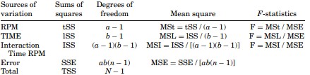
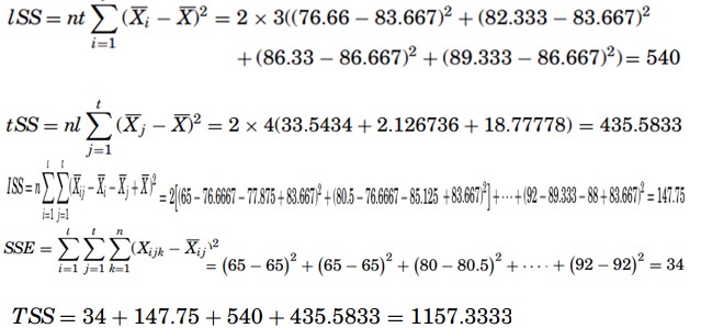
The formulas for the sums of squares (or deviations from means) to solve a two-way ANOVA with interaction are given as
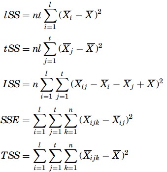
where lSS is the sum of squares for the rows, tSS is the sum of squares for the treatments, ISS is the sum of squares for the interactions, SSE is the error of the sum of squares, TSS is the total sum of squares, n is the number of observed data in a cell ( n = 2),t is the number of treatments, l is the number of row treatments, i is the number of treatment levels, j is the column treatment levels, k is the number of cells, Xijk is any observation, Xij is the cell mean, Xi is the level mean, Xj is the treatment mean, and X is the mean of all the observations. The table with the means of the numbers is added and the final table is as
| Hours | 500RPM | 550RPM | 600RPM | |
| 1 | 65 | 80 | 84 | |
| 65 | 81 | 85 | 76.66667 | |
| 2 | 75 | 83 | 85 | |
| 80 | 85 | 86 | 82.33333 | |
| 3 | 80 | 86 | 90 | |
| 85 | 87 | 90 | 86.33333 | |
| 4 | 85 | 89 | 92 | |
| 88 | 90 | 92 | 89.33333 |
The F-table with F-statistic is as
| Sources of variation | Sums of squares | Degrees of freedom | Mean square | F-statistic | F-critical |
| RPM | 435.45 | 2 | 217.79 | 76.86 | 3.89 |
| TIME | 540 | 3 | 180 | 63.53 | 3.49 |
| Interaction Time RPM | 147.75 | 6 | 24 | 8.69 | 3 |
| Error | 34 | 12 | 2.833 | ||
| Total | 1157.333 | 23 |
To reject the null hypothesis, compare the F-statistic to the F-critical value. If the F-critical value (the one on the F-table) is greater than the F-statistic (the calculated), do not reject the null hypothesis else, do it. In this case, the F-statistics for all the main factors and interaction are greater than their corresponding F-critical values, so reject the null hypotheses. The length of time the generators are operating, the RPM variations, and the interaction of RPM and time have an impact on the heat that the generators produce. But after determining the interaction between the two main factors is significant, it is unnecessary to investigate the main factors.
Determination of the significance of results is based on the P-value. In this example, all the P-values are infinitesimal, much lower than 0.05, which confirms the conclusion made earlier i.e. the RPMs, the time, and interactions have an effect on the heat produced by the generators. But after knowing that the interaction between the two main factors is significant, it is unnecessary to investigate the main factors.
Factorial (2k) Designs – They are experiments involving several factors ( k = # of factors) where it is necessary to study the joint effect of these factors on a specific response. Each of the factors are set at two levels (a “low” level and a “high” level) which may be qualitative (machine A/machine B, fan on/fan off) or quantitative (temperature 800/temperature 900, line speed 4000 per hour/line speed 5000 per hour).
Factors are assumed to be fixed (fixed effects model) and designs are completely randomized (experimental trials are run in a random order, etc.). The usual normality assumptions are satisfied. Further, particularly useful in the early stages of experimental work when likely to have many factors being investigated and to minimize the number of treatment combinations (sample size) but, at the same time, study all k factors in a complete factorial arrangement (the experiment collects data at all possible combinations of factor levels). As k gets large, the sample size will increase exponentially. If experiment is replicated, the # runs again increases.
| k | No of runs |
| 2 | 4 |
| 3 | 8 |
| 4 | 16 |
| 5 | 32 |
Two factors set at two levels (normally referred to as low and high) would result in the following design where each level of factor A is paired with each level of factor B.
| Generalized Settings | |||
| RUN | Factor A | Factor B | Response |
| 1 | low | low | y1 |
| 2 | high | low | y2 |
| 3 | low | high | y3 |
| 4 | high | high | y4 |
| Orthogonal Settings | |||
| RUN | Factor A | Factor B | Response |
| 1 | -1 | -1 | y1 |
| 2 | +1 | +1 | y2 |
| 3 | -1 | +1 | y3 |
| 4 | +1 | -1 | y4 |
Estimating main effects associated with changing the level of each factor from low to high. This is the estimated effect on the response variable associated with changing factor A or B from their low to high values as
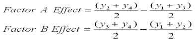
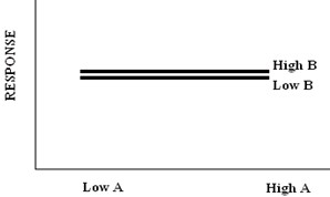
If neither factor A nor factor B have an effect on the response variable.
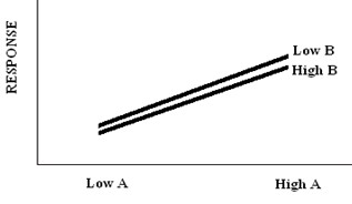
If factor A has an effect on the response variable, but factor B does not.
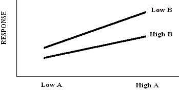
If factor A and factor B have an effect on the response variable.
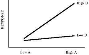
If factor B has an effect on the response variable, but only if factor A is set at the “High” level. This is called interaction and it basically means that the effect one factor has on a response is dependent on the level, being set other factors at. Interactions can be major problems in a DOE if fail to account for the interaction when designing experiment.