If the historical data are restricted to past values of the variable to be forecast, the forecasting procedure is called a time series method and the historical data are referred to as time series . The objective of time series analysis is to uncover a pattern in the time series and then extrapolate the pattern into the future; the forecast is based solely on past values of the variable and/or on past forecast errors.
A time series is a sequence of observations on a variable measured at successive points in time or over successive periods of time. The measurements may be taken every hour, day, week, month, year, or any other regular interval. The pattern of the data is an important factor in understanding how the time series has behaved in the past. If such behavior can be expected to continue in the future, we can use it to guide us in selecting an appropriate forecasting method.
To identify the underlying pattern in the data, a useful first step is to construct a time series plot, which is a graphical presentation of the relationship between time and the time series variable; time is represented on the horizontal axis and values of the time series variable are shown on the vertical axis. Let us first review some of the common types of data patterns that can be identified in a time series plot.
Time series graphs, a useful graphical way of displaying time series data. We use these time series graphs to help explain and identify four important components of a time series. These components are called the trend component, the seasonal component, the cyclic component, and the random (or noise) component.
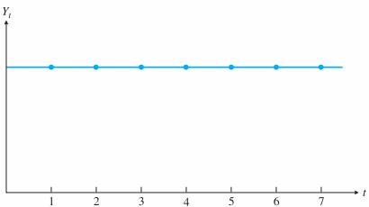
A time series where every observation has the same value. Such a series is shown in figure above. The graph in this figure shows time (t) on the horizontal axis and the observed values (Y ) on the vertical axis. We assume that Y is measured at regularly spaced intervals, usually days, weeks, months, quarters, or years, with Yt being the value of the observation at time period t. As indicated
in the figure, the individual observation points are usually joined by straight lines to make any patterns in the time series more apparent. Because all observations in this time series are equal, the resulting time series graph is a horizontal line. We refer to this time series as the base series.
Forecasting Time Series with a Linear Trend
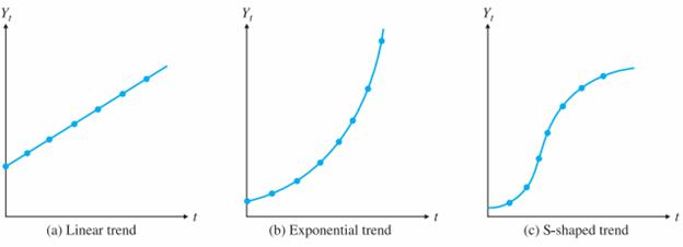
If the observations increase or decrease regularly through time, we say that the time series has a trend. The graphs in below figure illustrate several possible trends. The linear trend in the figure linear occurs if a company’s sales increase by the same amount from period to period. This constant per period change is then the slope of the linear trend line. The curve in exponential, occurs in a business such as the personal computer business, where sales have increased at a tremendous rate (at least during the 1990s, the boom years). For this type of curve, the percentage increase in Yt from period to period remains constant. The S-shaped curve, is appropriate for a new product that takes a while to catch on, then exhibits a rapid increase in sales as the public becomes aware of it, and initially tapers off to a fairly constant level because of market saturation. All the series in the figure represent upward trends and there are downward trends of the same types.
Forecasting Time Series with Seasonality
Many time series have a seasonal component, that is, they exhibit seasonality. For example, a company’s sales of swimming pool equipment increase every spring, then stay relatively high during the summer, and then drop off until next spring, at which time the yearly pattern repeats itself. An important aspect of the seasonal component is that it tends to be predictable from one year to the next. That is, the same seasonal pattern tends to repeat itself every year.
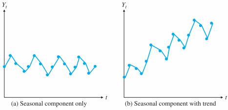
Seasonal patterns are recognized by observing recurring patterns over successive periods of time. For example, a manufacturer of swimming pools expects low sales activity in the fall and winter months, with peak sales in the spring and summer months to occur every year. Some time series include both a trend and a seasonal pattern.
Cyclical Pattern
A cyclical pattern exists if the time series plot shows an alternating sequence of points below and above the trendline that lasts for more than one year. Many economic time series exhibit cyclical behavior with regular runs of observations below and above the trendline. Often the cyclical component of a time series is due to multiyear business cycles. For example, periods of moderate inflation followed by periods of rapid inflation can lead to a time series that alternates below and above a generally increasing trendline (e.g., a time series for housing costs). Business cycles are extremely difficult, if not impossible, to forecast. As a result, cyclical effects are often combined with long-term trend effects and referred to as trend-cycle effects . In this chapter we do not deal with cyclical effects that may be present in the time series.
Random Pattern
Random variation, or simply noise, is an unpredictable component, which gives most time series graphs their irregular, zigzag appearance. Usually, a time series can be determined only to a certain extent by its trend, seasonal, and cyclic components. Then other factors determine the rest. These other factors may be inherent randomness, unpredictable “shocks” to the system, the unpredictable behavior of human beings who interact with the system, and possibly others. These factors combine to create a certain amount of unpredictability in almost all time series.
The Naive Methods
The forecasting methods covered under this category are mathematically very simple. The simplest of them uses the most recently observe d value in the time series as the forecast for the next period. Effectively, this implies that all prior observations are not considered. Another method of this type is the ‘free-hand projection method’.
This includes the plotting of the data series on a graph paper and fitting a free-hand curve to it. This curve is extended in to the future for deriving the forecasts. The ‘semi-average projection method’ is another naive method. Here, the time-series is divided into two equal halves, averages calculated for both, and a line drawn connecting the two semi averages. This line is projected into the future and the forecasts are developed.
Moving Averages Method
The moving averages method uses the average of the most recent k data values in the time series as the forecast for the next period. Mathematically, a moving average forecast of order k is
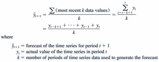
The term moving is used because every time a new observation becomes available for the time series, it replaces the oldest observation in the equation and a new average is computed. Thus, the periods over which the average is calculated change, or move, with each ensuing period.
To use moving averages to forecast a time series, we must first select the order k, or the number of time series values to be included in the moving average. If only the most recent values of the time series are considered relevant, a small value of k is preferred. If a greater number of past values are considered relevant, then we generally opt for a larger value of k. As previously mentioned, a time series with a horizontal pattern can shift to a new level over time. A moving average will adapt to the new level of the series and continue to provide good forecasts in k periods. Thus a smaller value of k will track shifts in a time series more quickly. On the other hand, larger values of k will be more effective in smoothing out random fluctuations. Thus, managerial judgment based on an understanding of the behavior of a time series is helpful in choosing an appropriate value of k.
Essentially, moving averages try to estimate the next period’s value by averaging the value of the last couple of periods immediately prior. Let’s say that you have been in business for three months, January through March, and wanted to forecast April’s sales. Sales for the last three months are as
| Month | Sales ($000) |
| January | 129 |
| February | 134 |
| March | 122 |
The simplest approach would be to take the average of January through March and use that to estimate April’s sales, as – (129 + 134 + 122)/3 = $128.333
Hence, based on the sales of January through March, you predict that sales in April will be $128,333. Once April’s actual sales come in, you would then compute the forecast for May, this time using February through April. You must be consistent with the number of periods you use for moving average forecasting.
The number of periods you use in your moving average forecasts are arbitrary; you may use only two-periods, or five or six periods – whatever you desire – to generate your forecasts.
The approach above is a simple moving average. Sometimes, more recent months’ sales may be stronger influencers of the coming month’s sales, so you want to give those nearer months more weight in your forecast model. This is a weighted moving average. And just like the number of periods, the weights you assign are purely arbitrary. Let’s say you wanted to give March’s sales 50% weight, February’s 30% weight, and January’s 20%. Then your forecast for April will be $127,000 [(122*.50) + (134*.30) + (129*.20) = 127].
Limitations – Moving averages are considered a “smoothing” forecast technique. Because you’re taking an average over time, you are softening (or smoothing out) the effects of irregular occurrences within the data. As a result, the effects of seasonality, business cycles, and other random events can dramatically increase forecast error. Take a look at a full year’s worth of data, and compare a 3-period moving average and a 5-period moving average:
| Month | Sales ($000) | 3-Mo. Moving Average | 5-Mo. Moving Average |
| January | 129 | ||
| February | 134 | 128.3 | |
| March | 122 | 127.0 | 128.2 |
| April | 125 | 126.0 | 129.8 |
| May | 131 | 131.0 | 128.6 |
| June | 137 | 132.0 | 130.4 |
| July | 128 | 132.0 | 129.2 |
| August | 131 | 126.0 | 127.8 |
| September | 119 | 124.7 | 126.0 |
| October | 124 | 123.7 | 127.6 |
| November | 128 | 129.3 | |
| December | 136 |
Notice that in this instance that no forecasts are created, but rather centered the moving averages. The first 3-month moving average is for February, and it’s the average of January, February, and March.
Weighted Moving Average Method
When using an “average” we are applying the same importance (weight) to each value in the dataset. In the 4-month moving average, each month represented 25% of the moving average. When using demand history to project future demand (and especially future trend), it’s logical to come to the conclusion that you would like more recent history to have a greater impact on your forecast. We can adapt our moving-average calculation to apply various “weights” to each period to get our desired results. We express these weights as percentages, and the total of all weights for all periods must add up to 100%. Therefore, if we decide we want to apply 35% as the weight for the nearest period in our 4-month “weighted moving average”, we can subtract 35% from 100% to find we have 65% remaining to split over the other 3 periods. For example, we may end up with a weighting of 15%, 20%, 30%, and 35% respectively for the 4 months (15 + 20 + 30 + 35 = 100).
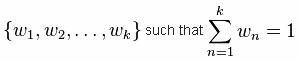
It is a slightly more intricate method for smoothing a raw time series {xt} is to calculate a weighted moving average by first choosing a set of weighting factors
and then using these weights to calculate the smoothed statistics {st}:
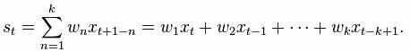
In practice the weighting factors are often chosen to give more weight to the most recent terms in the time series and less weight to older data. Notice that this technique has the same disadvantage as the simple moving average technique (i.e., it cannot be used until at least k observations have been made), and that it entails a more complicated calculation at each step of the smoothing procedure. In addition to this disadvantage, if the data from each stage of the averaging is not available for analysis, it may be difficult if not impossible to reconstruct a changing signal accurately (because older samples may be given less weight). If the number of stages missed is known however, the weighting of values in the average can be adjusted to give equal weight to all missed samples to avoid this issue.
Exponential Smoothing Method
If we go back to the concept of applying a weight to the most recent period (such as 35% in the previous example) and spreading the remaining weight (calculated by subtracting the most recent period weight of 35% from 100% to get 65%), we have the basic building blocks for our exponential smoothing calculation. The controlling input of the exponential smoothing calculation is known as the smoothing factor (also called the smoothing constant). It essentially represents the weighting applied to the most recent period’s demand. So, where we used 35% as the weighting for the most recent period in the weighted moving average calculation, we could also choose to use 35% as the smoothing factor in our exponential smoothing calculation to get a similar effect. The difference with the exponential smoothing calculation is that instead of us having to also figure out how much weight to apply to each previous period, the smoothing factor is used to automatically do that.
So here comes the “exponential” part. If we use 35% as the smoothing factor, the weighting of the most recent period’s demand will be 35%. The weighting of the next most recent period’s demand (the period before the most recent) will be 65% of 35% (65% comes from subtracting 35% from 100%). This equates to 22.75% weighting for that period if you do the math.
The next most recent period’s demand will be 65% of 65% of 35%, which equates to 14.79%. The period before that will be weighted as 65% of 65% of 65% of 35%, which equates to 9.61%, and so on. And this goes on back through all your previous periods all the way back to the beginning of time (or the point at which you started using exponential smoothing for that particular item).
You’re probably thinking that’s looking like a whole lot of math. But the beauty of the exponential smoothing calculation is that rather than having to recalculate against each previous period every time you get a new period’s demand, you simply use the output of the exponential smoothing calculation from the previous period to represent all previous periods.
Typically we refer to the output of the exponential smoothing calculation as the next period “forecast”. In reality, the ultimate forecast needs a little more work, but for the purposes of this specific calculation, we will refer to it as the forecast.
The exponential smoothing calculation is as follows:
The most recent period’s demand multiplied by the smoothing factor.
PLUS
The most recent period’s forecast multiplied by (one minus the smoothing factor).
OR
(D*S)+(F*(1-S))
Where
D = most recent period’s demand
S = the smoothing factor represented in decimal form (so 35% would be represented as 0.35).
F = the most recent period’s forecast (the output of the smoothing calculation from the previous period).
OR (assuming a smoothing factor of 0.35)
(D * 0.35) + ( F * 0.65)
As you can see, all we need for data inputs here are the most recent period’s demand and the most recent period’s forecast. We apply the smoothing factor (weighting) to the most recent period’s demand the same way we would in the weighted moving average calculation. We then apply the remaining weighting (1 minus the smoothing factor) to the most recent period’s forecast.
Since the most recent period’s forecast was created based on the previous period’s demand and the previous period’s forecast, which was based on the demand for the period before that and the forecast for the period before that, which was based on the demand for the period before that and the forecast for the period before that, which was based on the period before that . . .
The method only needs three numbers
- Ft-1 = Forecast for the period before current time period t
- At-1 = Actual demand for the period before current time period t
- a = Weight between 0 and 1
Formula
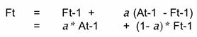
As a gets closer to 1, the more weight put on the most recent demand number
