Causal or exploratory forecasting methods are based on the assumption that the variable we are forecasting has a cause-effect relationship with one or more other variables. These methods help explain how the value of one variable impacts the value of another. For instance, the sales volume for many products is influenced by advertising expenditures, so regression analysis may be used to develop an equation showing how these two variables are related. Then, once the advertising budget is set for the next period, we could substitute this value into the equation to develop a prediction or forecast of the sales volume for that period. If a time series method was used to develop the forecast, advertising expenditures would not be considered; that is, a time series method would base the forecast solely on past sales.
Econometric Models
Econometric models, also called causal or regression-based models, use regression to forecast a time series variable by using other explanatory time series variables. For example, a company might use a causal model to regress future sales on its advertising level, the population income level, the interest rate, and possibly others. In one sense, regression analysis involving time series variables is similar to the regression analysis discussed in the previous two chapters. The same least squares approach and the same multiple regression software can be used in many time series regression models.
Suppose a company wants to use a regression model to forecast its monthly sales for some product, using two other time series variables as predictors: its monthly advertising levels for the product and its main competitor’s monthly advertising levels for a competing product. The resulting regression equation has the form
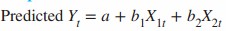
Here, Yt is the company’s sales in month t, and X1t and X2t are, respectively, the company’s and the competitor’s advertising levels in month t. This regression model might provide some useful results, but there are some issues that must be faced.
One issue is that the appropriate “lags” for the regression equation must be determined. Do sales this month depend only on advertising levels this month, as specified in the equation, or also on advertising levels in the previous month, the previous two months, and so on?
A second issue is whether to include lags of the sales variable in the regression equation as explanatory variables. Presumably, sales in one month might depend on the level of sales in previous months (as well as on advertising levels). A third issue is that the two advertising variables can be auto-correlated and cross-correlated. Autocorrelation means correlated with itself. For example, the company’s advertising level in one month might depend on its advertising levels in previous months. Cross-correlation means being correlated with a lagged version of another variable. For example, the company’s advertising level in one month might be related to the competitor’s advertising levels in previous months, or the competitor’s advertising in one month might be related to the company’s advertising levels in previous months.
These are difficult issues, and the way in which they are addressed can make a big difference in the usefulness of the regression model.
Linear Trend Projection
Regression analysis can be used to forecast a time series with a linear trend. Although the time series plot shows some up-and-down movement over the past ten years, we might agree that the linear trendline provides a reasonable approximation of the long-run movement in the series.
When a time series reflects a shift from a stationary pattern to real growth or decline in the time series variable of interest (e.g., product demand or student enrollment at the university), that time series is demonstrating the trend component. The trend projection method of time series forecasting is based on the simple linear regression model. However, we generally do not require the rigid assumptions of linear regression (normal distribution of the error component, constant variance of the error component, and so forth), only that the past linear trend pattern will continue into the future. Trend pattern reflects a curve, we would have to rely on the more sophisticated features of multiple regression.
The linear regression line is of the form Y = a + bX , where Y is the value of the de pendent variable that we are solving for, a is the Y intercept, b is the slope, and X is the independent variable. (In time series analysis, X is un its of time )
Linear regression is useful for long term forecasting of major occurrences and aggregate planning. For e x ample, linear regression would be very useful to forecast demands for product families. Even though demand for individual products within a family may vary widely during a time period, demand for the total product family is surprisingly smooth.
The major restriction in using linear regression forecasting is, as the name implies, that past data and future projections are assumed to fall about a straight line. Although this does limit its application, sometimes, if we use a shorter period of time, linear regression analysis can still be used. For example, there may be short segments of the longer period that are approximately linear.
Linear regression is used both for time series forecasting and for casual relationship forecasting . When the dependent variable (usually the vertical axis on the graph) changes as a result of time (plotted on the horizontal axis), it is time series analysis. When the dependent variable changes because of the change in another variable, this is a casual relationship (such as the demand of cold drinks increasing with the temperature).
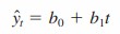
We can use regression analysis to develop such a linear trendline for the sales time series. Because simple linear regression analysis yields the linear relationship between the independent variable and the dependent variable that minimizes the mean square of error, we can use this approach to find a best-fitting line to a set of data that exhibits a linear trend. In finding a linear trend, the variable to be forecasted (y, the actual value of the time series period t) is the dependent variable and the trend variable (time period t) is the independent variable. We will use the following notation for our linear trendline.
Where,
y^ = forecast of sales in period t
t = time period
b0 = the y-intercept of the linear trendline
b1 = the slope of the linear trendline
Least Squares Regression
Linear Regression or Least Squares Regression (LSR) is the most popular method for identifying a linear trend in historical sales data. The method calculates the values for “a” and “b” to be used in the formula: Y = a + bX. The equation describes a straight line where Y represents sales, and X represents time. Linear regression is slow to recognize turning points and step function shifts in demand. Linear regression fits a straight line to the data, even when the data is seasonal or would better be described by a curve. When the sales history data follows a curve or has a strong seasonal pattern, forecast bias and systematic errors occur.
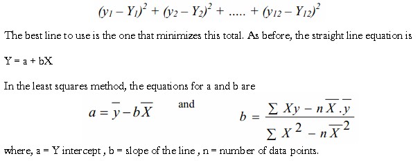
The least square method tries to fit the line to the data that minimizes the sum of the squares of the vertical distance between each data point and its corresponding point on the line.
If a straight line is drawn through general area of the points, the difference between the point and the line is y – Y. The sum of the squares of the differences between the plotted data points and the line point s is