Simulation
Simulation is the imitation of the operation of a real-world process or system over time. The act of simulating something first requires that a model be developed; this model represents the key characteristics or behaviors/functions of the selected physical or abstract system or process. The model represents the system itself, whereas the simulation represents the operation of the system over time.
Simulation is used in many contexts, such as simulation of technology for performance optimization, safety engineering, testing, training, education, and video games. Often, computer experiments are used to study simulation models. Simulation is also used with scientific modeling of natural systems or human systems to gain insight into their functioning. Simulation can be used to show the eventual real effects of alternative conditions and courses of action. Simulation is also used when the real system cannot be engaged, because it may not be accessible, or it may be dangerous or unacceptable to engage, or it is being designed but not yet built, or it may simply not exist.
Risk analysis is a technique used to identify and assess factors that may jeopardize the success of a project or achieving a goal.
This technique also helps to define preventive measures to reduce the probability of these factors from occurring and identify countermeasures to successfully deal with these constraints when they develop to avert possible negative effects on the competitiveness of the company.
Risk Analysis
Risk analysis is a technique used to identify and assess factors that may jeopardize the success of a project or achieving a goal.
This technique also helps to define preventive measures to reduce the probability of these factors from occurring and identify countermeasures to successfully deal with these constraints when they develop to avert possible negative effects on the competitiveness of the company.
Risk analysis can be “broadly defined to include risk assessment, risk characterization, risk communication, risk management, and policy relating to risk, in the context of risks of concern to individuals, to public- and private-sector organizations, and to society at a local, regional, national, or global level.” A useful construct is to divide risk analysis into two components: (1) risk assessment (identifying, evaluating, and measuring the probability and severity of risks) and (2) risk management (deciding what to do about risks)
Monte Carlo methods (or Monte Carlo experiments) are a broad class of computational algorithms that rely on repeated random sampling to obtain numerical results. They are often used when it is difficult or impossible to use other mathematical methods. Monte Carlo methods are mainly used in three distinct problem classes: optimization, numerical integration, and generating draws from a probability distribution.
In principle, Monte Carlo methods can be used to solve any problem having a probabilistic interpretation. By the law of large numbers, integrals described by the expected value of some random variable can be approximated by taking the empirical mean (a.k.a. the sample mean) of independent samples of the variable.
Monte Carlo methods vary, but tend to follow a particular pattern:
- Define a domain of possible inputs.
- Generate inputs randomly from a probability distribution over the domain.
- Perform a deterministic computation on the inputs.
- Aggregate the results.
For example, consider a circle inscribed in a unit square. Given that the circle and the square have a ratio of areas that is π/4, the value of π can be approximated using a Monte Carlo method:
- Draw a square on the ground, then inscribe a circle within it.
- Uniformly scatter some objects of uniform size (grains of rice or sand) over the square.
- Count the number of objects inside the circle and the total number of objects.
- The ratio of the two counts is an estimate of the ratio of the two areas, which is π/4. Multiply the result by 4 to estimate π.
In this procedure the domain of inputs is the square that circumscribes our circle. We generate random inputs by scattering grains over the square then perform a computation on each input (test whether it falls within the circle). Finally, we aggregate the results to obtain our final result, the approximation of π.
There are two important points to consider here: Firstly, if the grains are not uniformly distributed, then our approximation will be poor. Secondly, there should be a large number of inputs. The approximation is generally poor if only a few grains are randomly dropped into the whole square. On average, the approximation improves as more grains are dropped.
Uses of Monte Carlo methods require large amounts of random numbers, and it was their use that spurred the development of pseudorandom number generators, which were far quicker to use than the tables of random numbers that had been previously used for statistical sampling.
Monte Carlo simulation uses repeated sampling to determine the properties of some phenomenon (or behavior). Examples:
- Simulation: Drawing one pseudo-random uniform variable from the interval [0,1] can be used to simulate the tossing of a coin: If the value is less than or equal to 0.50 designate the outcome as heads, but if the value is greater than 0.50 designate the outcome as tails. This is a simulation, but not a Monte Carlo simulation.
- Monte Carlo method: Pouring out a box of coins on a table, and then computing the ratio of coins that land heads versus tails is a Monte Carlo method of determining the behavior of repeated coin tosses, but it is not a simulation.
- Monte Carlo simulation: Drawing a large number of pseudo-random uniform variables from the interval [0,1], and assigning values less than or equal to 0.50 as heads and greater than 0.50 as tails, is a Monte Carlo simulation of the behavior of repeatedly tossing a coin.
Whenever you need to make an estimate, forecast or decision where there is significant uncertainty, you’d be well advised to consider Monte Carlo simulation — if you don’t, your estimates or forecasts could be way off the mark, with adverse consequences for your decisions! Dr. Sam Savage, a noted authority on simulation and other quantitative methods, says “Many people, when faced with an uncertainty … succumb to the temptation of replacing the uncertain number in question with a single average value. I call this the flaw of averages, and it is a fallacy as fundamental as the belief that the earth is flat.”
Most business activities, plans and processes are too complex for an analytical solution — just like the physics problems of the 1940s. But you can build a spreadsheet model that lets you evaluate your plan numerically — you can change numbers, ask ‘what if’ and see the results. This is straightforward if you have just one or two parameters to explore. But many business situations involve uncertainty in many dimensions — for example, variable market demand, unknown plans of competitors, uncertainty in costs, and many others — just like the physics problems in the 1940s. If your situation sounds like this, you may find that the Monte Carlo method is surprisingly effective for you as well.
To use Monte Carlo simulation, you must be able to build a quantitative model of your business activity, plan or process. To deal with uncertainties in your model, replace certain fixed numbers with functions that draw random samples from probability distributions. By exploring thousands of combinations for your ‘what-if’ factors and analyzing the full range of possible outcomes, you can get much more accurate results, with only a little extra work.
Example: Rolling Dice
As a simple example of a Monte Carlo simulation, consider calculating the probability of a particular sum of the throw of two dice (with each die having values one through six). In this particular case, there are 36 combinations of dice rolls:
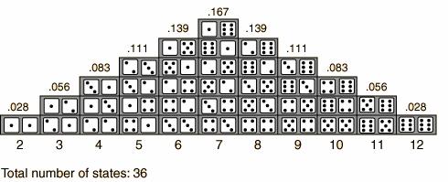
Based on this, you can manually compute the probability of a particular outcome. For example, there are six different ways that the dice could sum to seven. Hence, the probability of rolling seven is equal to 6 divided by 36 = 0.167.
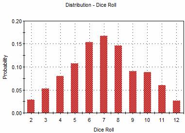
Instead of computing the probability in this way, however, we could instead throw the dice a hundred times and record how many times each outcome occurs. If the dice totaled seven 18 times (out of 100 rolls), we would conclude that the probability of rolling seven is approximately 0.18 (18%). Obviously, the more times we rolled the dice, the less approximate our result would be. Better than rolling dice a hundred times, we can easily use a computer to simulate rolling the dice 10,000 times (or more). Because we know the probability of a particular outcome for one die (1 in 6 for all six numbers), this is simple. The output of 10,000 realizations are
Results Accuracy – The accuracy of a Monte Carlo simulation is a function of the number of realizations. That is, the confidence bounds on the results can be readily computed based on the number of realizations. The two examples below show the 5% and 95% confidence bounds on the value for each outcome (i.e., there is a 90% chance the true value lies between the bounds)
