
Hypothesis Testing- A hypothesis is a theory about the relationships between variables. Statistical analysis is used to determine if the observed differences between two or more samples are due to random chance or to true differences in the samples.
Basics
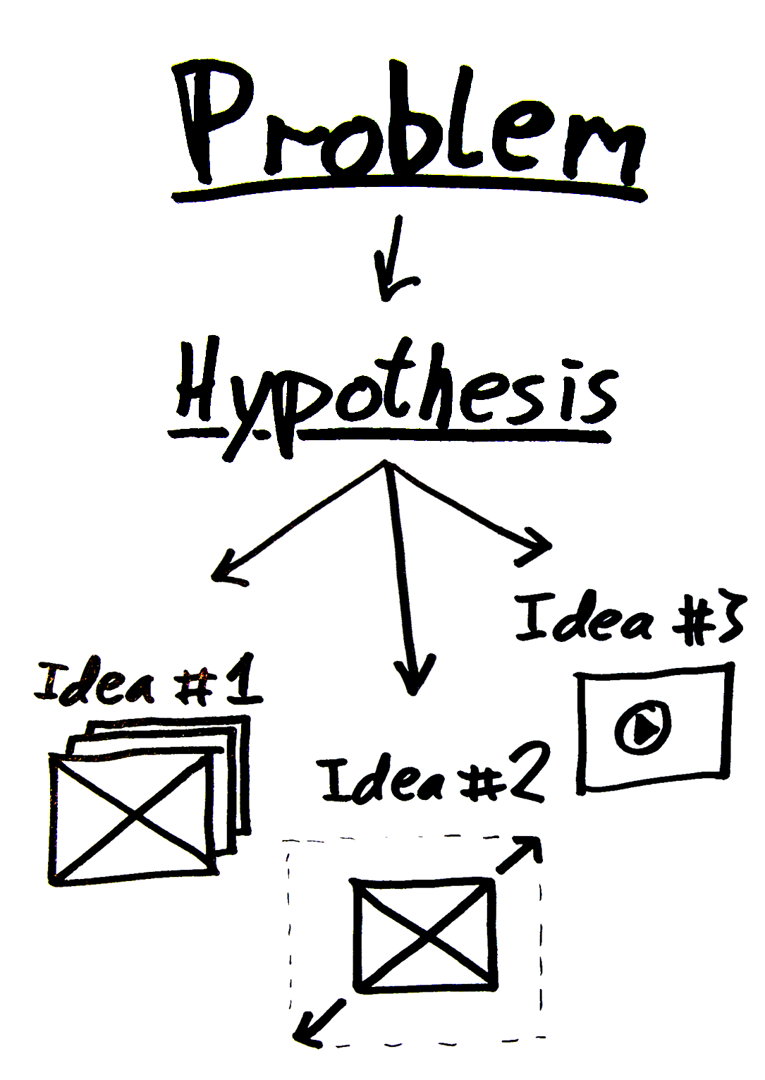
Hypothesis Testing- A hypothesis is a value judgment, a statement based on an opinion about a population. It is developed to make an inference about that population. Based on experience, a design engineer can make a hypothesis about the performance or qualities of the products she is about to produce, but the validity of that hypothesis must be ascertained to confirm that the products are produced to the customer’s specifications. A test must be conducted to determine if the empirical evidence does support the hypothesis.
Practical Significance – Practical significance is the amount of difference, change or improvement that will add practical, economic or technical value to an organization.
Statistical Significance – Statistical significance is the magnitude of difference or change required to distinguish between a true difference, change or improvement and one that could have occurred by chance. The larger the sample size, the more likely the observed difference is close to the actual difference.
Null– The first step consists in stating the hypothesis. It is denoted by H0, and is read “H sub zero.” The statement will be written as H0: µ = 20%. A null hypothesis assumes no difference exists between or among the parameters being tested and is often the opposite of what is hoped to be proven through the testing. The null hypothesis is typically represented by the symbol Ho.
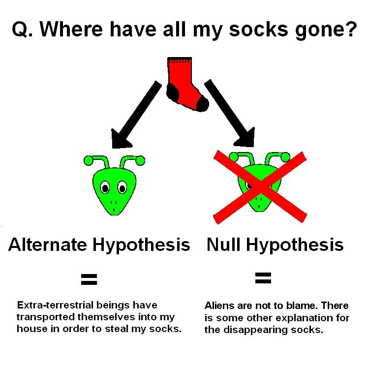
Alternate Hypothesis – If the hypothesis is not rejected, exactly 20 percent of the defects will actually be traced to the CPU socket. But if enough evidence is statistically provided that the null hypothesis is untrue, an alternate hypothesis should be assumed to be true. That alternate hypothesis, denoted H1, tells what should be concluded if H0 is rejected. H1 : µ ≠ 20%. An alternate hypothesis assumes that at least one difference exists between or among the parameters being tested. This hypothesis is typically represented by the symbol Ha.
Test Statistic – The decision made on whether to reject H0 or fail to reject it depends on the information provided by the sample taken from the population being studied. The objective here is to generate a single number that will be compared to H0 for rejection. That number is called the test statistic.
The level of risk – It addresses the risk of failing to reject a hypothesis when it is actually false, or rejecting a hypothesis when it is actually true.
Type I error (False Positive) – It occurs when one rejects the null hypothesis when it is true. The probability of a type I error is the level of significance of the test of hypothesis, and is denoted by *alpha*. Usually a one-tailed test of hypothesis is used when one talks about type I error or alpha error.
Type II error (False Negative) – It occurs when one rejects the alternative hypothesis (fails to reject the null hypothesis) when the alternative hypothesis is true. The probability of a type II error is denoted by *beta*.
Decision Rule Determination – The decision rule determines the conditions under which the null hypothesis is rejected or not. The critical value is the dividing point between the area where H0 is rejected and the area where it is assumed to be true.
Decision Making – Only two decisions are considered, either the null hypothesis is rejected or it is not. The decision to reject a null hypothesis or not depends on the level of significance. This level often varies between 0.01 and 0.10. Even when we fail to reject the null hypothesis, we never say “we accept the null hypothesis” because failing to reject the null hypothesis that was assumed true does not equate proving its validity.
Testing for a Population Mean – When the sample size is greater than 30 and σ is known, the Z formula can be used to test a null hypothesis about the mean.
Phrasing – In hypothesis, the phrase “to accept” the null hypothesis is not typically used. In statistical terms, the Six Sigma Black Belt can reject the null hypothesis, thus accepting the alternate hypothesis, or fail to reject the null hypothesis. This phrasing is similar to jury’s stating that the defendant is not guilty, not that the defendant is innocent.
One Tail Test – In a one-tailed t-test, all the area associated with a is placed in either one tail or the other. Selection of the tail depends upon which direction to bs would be (+ or -) if the results of the experiment came out as expected. The selection of the tail must be made before the experiment is conducted and analyzed.
Sample Size – It has been assumed that the sample size (n) for hypothesis testing has been given and that the critical value of the test statistic will be determined based on the error that can be tolerated.
Paired-Comparison Tests
They are powerful ways to compare data sets by determining if the means of the paired samples are equal. Making both measurements on each unit in a sample allows testing on the paired differences. An example of a paired comparison is two different types of hardness tests conducted on the same sample.
Once paired, a test of significance attempts to determine if the observed difference indicates whether the characteristics of the two groups are the same or different. A paired comparison experiment is an effective way to reduce the natural variability that exists among subjects and tests the null hypothesis that the average of the differences between a series of paired observations is zero.
Goodness of Fit – GOF (Goodness of Fit) tests are part of a class of procedures that are structured in cells. In each cell there is an observed frequency. In the goodness-of-fit tests, one is comparing and observed (O) frequency distribution to an expected (E) frequency distribution. The relationship is statistically described by a hypothesis test
- Ho: Random variable is distributed as a specific distribution with given parameters.
- Ha: Random variable does not have the specific distribution with given parameters.
Hypothesis Testing- Single-factor analysis of variance (ANOVA)
Sometimes it is essential to compare three or more population means at once with the assumptions as the variance is the same for all factor treatments or levels, the individual measurements within each treatment are normally distributed and the error term is considered a normally and independently distributed random effect. With analysis of variance, the variations in response measurement are partitioned into components that reflect the effects of one or more independent variables. The variability of a set of measurements is proportional to the sum of squares of deviations used to calculate the variance
ANOVA is a technique to determine if there are statistically significant differences among group means by analyzing group variances. An ANOVA is an analysis technique that evaluates the importance of several factors of a set of data by subdividing the variation into component parts. ANOVA tests to determine if the means are different, not which of the means are different Ho: μ1= μ2= μ3 and Ha: At least one of the group means is different from the others.
One-Way ANOVA
Terms used in ANOVA
- Degrees of Freedom (df) – The number of independent conclusions that can be drawn from the data.
- SSFactor – It measures the variation of each group mean to the overall mean across all groups.
- SSError – It measures the variation of each observation within each factor level to the mean of the level.
- Mean Square Error (MSE) – It is SSError/ df and is also the variance.
- F-test statistic – The ratio of the variance between treatments to the variance within treatments = MS/MSE. If F is near 1, then the treatment means are no different (p-value is large).
- P-value – It is the smallest level of significance that would lead to rejection of the null hypothesis (Ho). If α = 0.05 and the p-value ≤ 0.05, then reject the null hypothesis and conclude that there is a significant difference and if α = 0.05 and the p-value > 0.05, then fail to reject the null hypothesis and conclude that there is not a significant difference.
One-way ANOVA is used to determine whether data from three or more populations formed by treatment options from a single factor designed experiment indicate the population means are different. The assumptions in using One-way ANOVA is all samples are random samples from their respective populations and are independent, distributions of outputs for all treatment levels follow the normal distribution and equal or homogeneity of variances.
ANOVA Example –
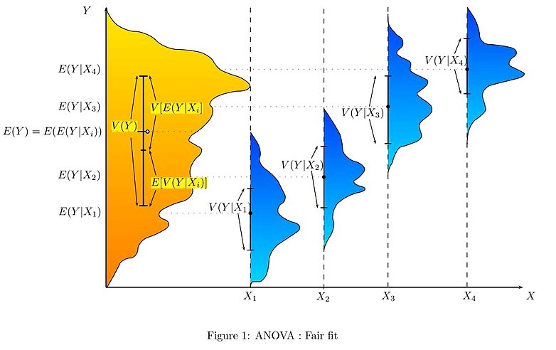
Hypothesis Testing- The analysis of variance can be used as an exploratory tool to explain observations. A dog show provides an example. A dog show is not a random sampling of the breed: it is typically limited to dogs that are male, adult, pure-bred, and exemplary. A histogram of dog weights from a show might plausibly be rather complex, like the yellow-orange distribution shown in the illustrations. Suppose we wanted to predict the weight of a dog based on a certain set of characteristics of each dog. Before we could do that, we would need to explain the distribution of weights by dividing the dog population into groups based on those characteristics. A successful grouping will split dogs such that a) each group has a low variance of dog weights (meaning the group is relatively homogeneous) and b) the mean of each group is distinct (if two groups have the same mean, then it isn’t reasonable to conclude that the groups are, in fact, separate in any meaningful way).
In the illustrations to the right, each group is identified as X1, X2, etc. In the first illustration, we divide the dogs according to the product (interaction) of two binary groupings: young vs old, and short-haired vs long-haired (thus, group 1 is young, short-haired dogs, group 2 is young, long-haired dogs, etc.). Since the distributions of dog weight within each of the groups (shown in blue) has a large variance, and since the means are very close across groups, grouping dogs by these characteristics does not produce an effective way to explain the variation in dog weights: knowing which group a dog is in does not allow us to make any reasonable statements as to what that dog’s weight is likely to be. Thus, this grouping fails to fit the distribution we are trying to explain (yellow-orange).
An attempt to explain the weight distribution by grouping dogs as (pet vs working breed) and (less athletic vs more athletic) would probably be somewhat more successful (fair fit). The heaviest show dogs are likely to be big strong working breeds, while breeds kept as pets tend to be smaller and thus lighter. As shown by the second illustration, the distributions have variances that are considerably smaller than in the first case, and the means are more reasonably distinguishable. However, the significant overlap of distributions, for example, means that we cannot reliably say that X1 and X2 are truly distinct (i.e., it is perhaps reasonably likely that splitting dogs according to the flip of a coin—by pure chance—might produce distributions that look similar).
An attempt to explain weight by breed is likely to produce a very good fit. All Chihuahuas are light and all St. Bernards are heavy. The difference in weights between Setters and Pointers does not justify separate breeds. The analysis of variance provides the formal tools to justify these intuitive judgments. A common use of the method is the analysis of experimental data or the development of models. The method has some advantages over correlation: not all of the data must be numeric and one result of the method is a judgment in the confidence in an explanatory relationship.
Hypothesis Testing- Chi square
Usually the objective of the project team is not to find the mean of a population but rather to determine the level of variation of the output like to know how much variation the production process exhibits about the target to see what adjustments are needed to reach a defect-free process.
If the means of all possible samples are obtained and organized we can derive the sampling distribution of the means similarly for variances, the sampling distribution of the variances can be known but, the distribution of the means follows a normal distribution when the population is normally distributed or when the samples are greater than 30, the distribution of the variance follows a Chi square (χ2) distribution.
Chi-square cannot be negative because it is the square of a number. If it is equal to zero, all the compared categories would be identical, therefore chi-square is a one-tailed distribution. The null and alternate hypotheses will be H0: The distribution of quality of the products after the parts were changed is the same as before the parts were changed. H1: The distribution of the quality of the products after the parts were changed is different than it was before they were changed.
The chi square test is used to test a distribution observed in the field against another distribution determined by a null hypothesis. Being a statistical test, chi square can be expressed as a formula. When written in mathematical notation the formula is as –
When using the chi-square test, the researcher needs a clear idea of what is being investigating. It is customary to define the object of the research by writing an hypothesis. Chi square is then used to either prove or disprove the hypothesis.
Take Free Mock Test on Six Sigma Green Belt
Become Vskills Certified Six Green Belts Professional. Gain knowledge on the module “Hypothesis Testing”. Try the free practice test!!
Apply for the Certification Exam !!
Certified Six Sigma Green Belt Professional