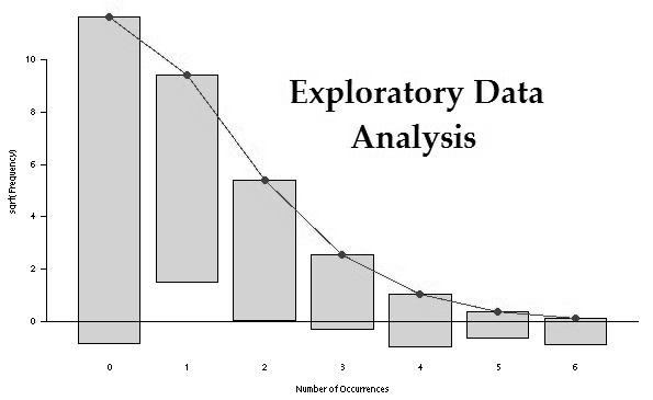
Exploratory data analysis or EDA, is the important first step in analyzing the data from an experiment as it is used for,
- Detection of mistakes
- Checking of assumptions
- Preliminary selection of appropriate models
- Determining relationships among the explanatory variables, and
- Assessing the direction and rough size of relationships between explanatory and outcome variables.
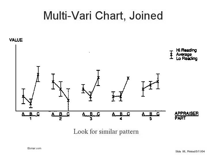
Multi-vari studies
Usually the variation is within piece and the source of this variation is different from piece-to-piece and time-to-time variation. Multi-vari charts are used to investigate the stability or consistency of a process.
The advantages of multi-vari charts are
- It can dramatize the variation within the piece (positional).
- It can dramatize the variation from piece to piece (cyclical).
- It helps to track any time related changes (temporal).
- It helps minimize variation by identifying areas to look for excessive variation. It also identifies areas not to look for excessive variation.
Sources of variation in multi-vari analysis can be
- Within Individual Sample – Variation is present upon repeat measurements within same sample.
- Piece to Piece – Variation is present upon measurements of different samples collected within a short time frame.
- Time to Time – Variation is present upon measurements collected with a significant amount of time between samples.
Multi-vari analysis is applicable to either product or service as it can control variation for both as,
- Within Individual Sample variations like Measurement Accuracy, Out of Round, Irregularities in Part, Measurement Accuracy and Line Item Complexity
- Piece to Piece variations like Machine fixturing, Mold cavity differences, Customer Differences, Order Editor, Sales Office and Sales Rep
- Time to Time variations like Material Changes, Setup Differences, Tool Wear, Calibration Drift, Operator Influence, Seasonal Variation, Management Changes, Economic Shifts and Interest Rate
Simple linear correlation and regression
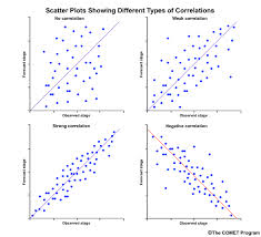
Correlation
Correlation is tool that is with a continuous x and a continuous y. The Pearson correlation coefficient (r) measures the linear relationship between the x and y as discussed earlier.
Confidence in a relationship is computed both by the correlation coefficient and by the number of pairs in data. If there are very few pairs then the coefficient needs to be very close to 1 or –1 for it to be deemed ‘statistically significant’, but if there are many pairs then a coefficient closer to 0 can still be considered ‘highly significant’.
Linear Regression
When the input and output variables are both continuous and to see a relationship between the two variables, regression and correlation are used. Determining how the predicted or dependent variable (the response variable, the variable to be estimated) reacts to the variations of the predicator or independent variable (the variable that explains the change) involves first to determine any relationship between them and it’s importance. Regression analysis builds a mathematical model that helps making predictions about the impact of variable variations.
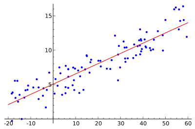
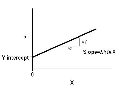
Exploratory Data Analysis- Linear regression consists of finding the best-fitting straight line through the points. The best-fitting line is called a regression line. The diagonal line in the figure is the regression line and consists of the predicted score on Y for each possible value of X. The vertical lines from the points to the regression line represent the errors of prediction. As the line from 1.00 is very near the regression line; its error of prediction is small and similarly for the line from 1.75 is much higher than the regression line and therefore its error of prediction is large.
Least Squares Method – In this method, for computing the values of b1 and b0, the vertical distance between each point and the line called the error of prediction is used. The line that generates the smallest error of predictions will be the least squares regression line.
Simple Linear Regression Hypothesis Testing
Hypothesis tests can be applied to determine whether the independent variable (x) is useful as a predictor for the dependent variable (y).
Multiple Linear Regression
Multiple linear regression expands on the simple linear regression model to allow for more than one independent or predictor variable. The general form for the equation is y = b0+ b1x + … bn+ e where, (b0,b1,b2…) are the coefficients and are referred to as partial regression coefficients. The equation may be interpreted as the amount of change in y for each unit increase in x (variable) when all other xs are held constant. The hypotheses for multiple regression are Ho:b1=b2= … =bn Ha:b1≠ 0 for at least one i.
Coefficient of Determination
Coefficients are estimated by minimizing the sum of squares (SS) residuals. The coefficients follow a t-distribution, which allows us to use t-tests to assess their significance. The coefficient of determination, R2, or multiple regression coefficients, is the proportion of variation in Y that can be explained by the regression model and is the square of r.
Take Free Mock Test on Six Sigma Green Belt
Become Vskills Certified Six Green Belts Professional. Gain knowledge on the module “Exploratory Data Analysis”. Try the free practice test!
Apply for the Certification Exam !!
Certified Six Sigma Green Belt Professional