It is the problem of optimizing (minimizing or maximizing) a quadratic function of several variables subject to linear constraints on these variables. It has an objective which is a quadratic function of the decision variables, and constraints which are all linear functions of the variables. An example of a quadratic function is
where X1, X2 and X3 are decision variables. A widely used QP problem is the Markowitz mean-variance portfolio optimization problem, where the quadratic objective is the portfolio variance (sum of the variances and co-variances of individual securities), and the linear constraints specify a lower bound for portfolio return.
QP problems, like LP problems, have only one feasible region with “flat faces” on its surface (due to the linear constraints), but the optimal solution may be found anywhere within the region or on its surface. The quadratic objective function may be convex — which makes the problem easy to solve — or non-convex, which makes it very difficult to solve.
The “best” QPs have Hessians that are positive definite (in a minimization problem) or negative definite (in a maximization problem). You can picture the graph of these functions as having a “round bowl” shape with a single bottom (or top) — a convex function. Portfolio optimization problems are usually of this type.
A QP with a semi-definite Hessian is still convex: It has a bowl shape with a “trough” where many points have the same objective value. An optimizer will normally find a point in the “trough” with the best objective function value.
A QP with an indefinite Hessian has a “saddle” shape — a non-convex function. Its true minimum or maximum is not found in the “interior” of the function but on its boundaries with the constraints, where there may be many locally optimal points. Optimizing an indefinite quadratic function is a difficult global optimization problem, and is outside the scope of most specialized quadratic solvers.
Definition
The quadratic programming problem with n variables and m constraints can be formulated as follows. Given:
- a real-valued, n-dimensional vector c,
- an n × n-dimensional real symmetric matrix Q,
- an m × n-dimensional real matrix A, and
- an m-dimensional real vector b,
the objective of quadratic programming is to find an n-dimensional vector x, that
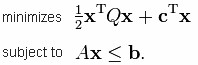
where xT denotes the vector transpose of x. The notation Ax ≤ b means that every entry of the vector Ax is less than or equal to the corresponding entry of the vector b.
A related programming problem, quadratically constrained quadratic programming, can be posed by adding quadratic constraints on the variables.
Solution Methods
For general problems a variety of methods are commonly used, including
- interior point
- active set
- augmented Lagrangian
- conjugate gradient
Interior point method
Interior point methods (also referred to as barrier methods) are a certain class of algorithms that solves linear and nonlinear convex optimization problems. Contrary to the simplex method, it reaches a best solution by traversing the interior of the feasible region. The method can be generalized to convex programming based on a self-concordant barrier function used to encode the convex set. Any convex optimization problem can be transformed into minimizing (or maximizing) a linear function over a convex set by converting to the epigraph form.
The class of primal-dual path-following interior point methods is considered the most successful.
Primal-dual interior point method for nonlinear optimization – The primal-dual method’s idea is easy to demonstrate for constrained nonlinear optimization. For simplicity consider the all-inequality version of a nonlinear optimization problem:
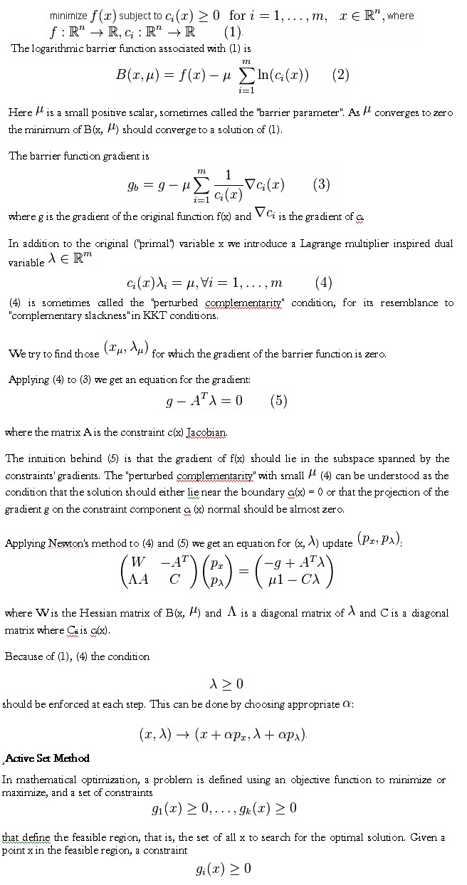
is called active at x if gi(x)=0 and inactive at x if gi(x)>0. Equality constraints are always active. The active set at x is made up of those constraints gi(x) that are active at the current point.
The active set is particularly important in optimization theory as it determines which constraints will influence the final result of optimization. For example, in solving the linear programming problem, the active set gives the hyperplanes that intersect at the solution point. In quadratic programming, as the solution is not necessarily on one of the edges of the bounding polygon, an estimation of the active set gives us a subset of inequalities to watch while searching the solution, which reduces the complexity of the search.
In general an active set algorithm has the following structure:
Find a feasible starting point
repeat until “optimal enough”
solve the equality problem defined by the active set (approximately)
compute the Lagrange multipliers of the active set
remove a subset of the constraints with negative Lagrange multipliers
search for infeasible constraints
end repeat
Augmented Lagrangian Method
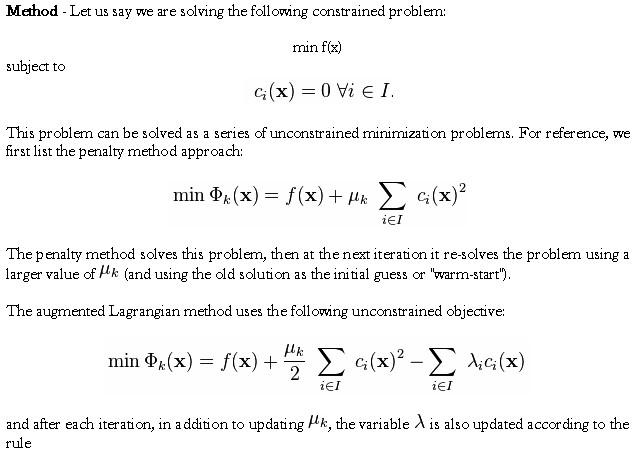
Augmented Lagrangian methods are a certain class of algorithms for solving constrained optimization problems. They have similarities to penalty methods in that they replace a constrained optimization problem by a series of unconstrained problems and add a penalty term to the objective; the difference is that the augmented Lagrangian method adds yet another term, designed to mimic a Lagrange multiplier. The augmented Lagrangian is not the same as the method of Lagrange multipliers.
Viewed differently, the unconstrained objective is the Lagrangian of the constrained problem, with an additional penalty term (the augmentation).
The method was originally known as the method of multipliers, and was studied much in the 1970 and 1980s as a good alternative to penalty methods. It was first discussed by Magnus Hestenes in 1969 and by Powell in 1969. The method was studied by R. Tyrrell Rockafellar in relation to Fenchel duality, particularly in relation to proximal-point methods, Moreau–Yosida regularization, and maximal monotone operators: These methods were used in structural optimization. The method was also studied by Dimitri Bertsekas, notably in his 1982 book, together with extensions involving nonquadratic regularization functions, such as entropic regularization, which gives rise to the “exponential method of multipliers,” a method that handles inequality constraints with a twice differentiable augmented Lagrangian function.
Since the 1970s, sequential quadratic programming (SQP) and interior point methods (IPM) have had increasing attention, in part because they more easily use sparse matrix subroutines from numerical software libraries, and in part because IPMs have proven complexity results via the theory of self-concordant functions. The augmented Lagrangian method was rejuvenated by the optimization systems LANCELOT and AMPL, which allowed sparse matrix techniques to be used on seemingly dense but “partially separable” problems. The method is still useful for some problems. Around 2007, there was a resurgence of augmented Lagrangian methods in fields such as total-variation denoising and compressed sensing. In particular, a variant of the standard augmented Lagrangian method that uses partial updates (similar to the Gauss-Seidel method for solving linear equations) known as the alternating direction method of multipliers or ADMM gained some attention.
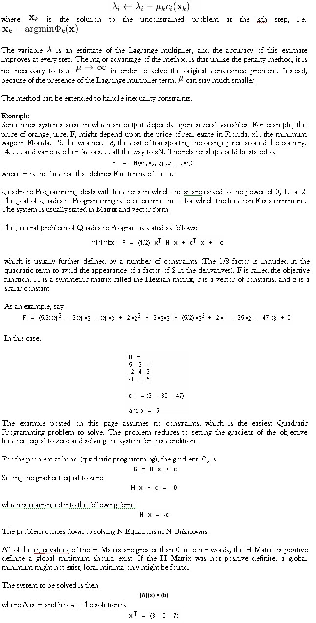
In other words, F takes a minimum value when
x1 = 3,
x2 = 5, and
x3 = 7
