Nonlinear programming (NP) involves minimizing or maximizing a nonlinear objective function subject to bound constraints, linear constraints, or nonlinear constraints, where the constraints can be inequalities or equalities. Example problems in engineering include analyzing design tradeoffs, selecting optimal designs, and incorporating optimization methods in algorithms and models.
Definition
Let n, m, and p be positive integers. Let X be a subset of Rn, let f, gi, and hj be real-valued functions on X for each i in {1, …, m} and each j in {1, …, p}.
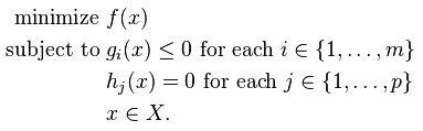
A nonlinear minimization problem is an optimization problem of the form.
Possible types of constraint set
There are several possibilities for the nature of the constraint set, also known as the feasible set or feasible region.
- An infeasible problem is one for which no set of values for the choice variables satisfy all the constraints. That is, the constraints are mutually contradictory, and no solution exists.
- A feasible problem is one for which there exists at least one set of values for the choice variables satisfying all the constraints.
- An unbounded problem is a feasible problem for which the objective function can be made to exceed any given finite value. Thus there is no optimal solution, because there is always a feasible solution that gives a better objective function value than does any given proposed solution.
Nonlinear models are inherently much more difficult to optimize due to following reasons
- It’s hard to distinguish a local optimum from a global optimum. Numerical methods for solving nonlinear programs have limited information about the problem, typically only information about the current point (and stored information about past points that have been visited).
- Optima are not restricted to extreme points. There are a limited number of places to look for the optimum in a linear program: we need only check the extreme point, or corner points, of the feasible region polytope.
- There may be multiple disconnected feasible regions. Because of the way in which nonlinear constraints can twist and curve, there may be multiple different feasible regions.
- Different starting points may lead to different final solutions.
- It may be difficult to find a feasible starting point.
- It is difficult to satisfy equality constraints (and to keep them satisfied).
- There is no definite determination of the outcome.
- There is a huge body of very complex mathematical theory and numerous solution algorithms.
- It is difficult to determine whether the conditions to apply a particular solver are met.
- Different algorithms and solvers arrive at different solutions (and outcomes) for the same formulation.
Solving Non-linear Optimization Problems
If the objective function f is linear and the constrained space is a polytope, the problem is a linear programming problem, which may be solved using well known linear programming solutions.
If the objective function is concave (maximization problem), or convex (minimization problem) and the constraint set is convex, then the program is called convex and general methods from convex optimization can be used in most cases.
If the objective function is a ratio of a concave and a convex function (in the maximization case) and the constraints are convex, then the problem can be transformed to a convex optimization problem using fractional programming techniques.
Several methods are available for solving nonconvex problems. One approach is to use special formulations of linear programming problems. Another method involves the use of branch and bound techniques, where the program is divided into subclasses to be solved with convex (minimization problem) or linear approximations that form a lower bound on the overall cost within the subdivision. With subsequent divisions, at some point an actual solution will be obtained whose cost is equal to the best lower bound obtained for any of the approximate solutions. This solution is optimal, although possibly not unique. The algorithm may also be stopped early, with the assurance that the best possible solution is within a tolerance from the best point found; such points are called ε-optimal. Terminating to ε-optimal points is typically necessary to ensure finite termination. This is especially useful for large, difficult problems and problems with uncertain costs or values where the uncertainty can be estimated with an appropriate reliability estimation.
Under differentiability and constraint qualifications, the Karush–Kuhn–Tucker (KKT) conditions provide necessary conditions for a solution to be optimal. Under convexity, these conditions are also sufficient. If some of the functions are non-differentiable, subdifferential versions of Karush–Kuhn–Tucker (KKT) conditions are available.
The following algorithms are commonly used for unconstrained nonlinear programming:
- Quasi-Newton: uses a mixed quadratic and cubic line search procedure and the Broyden-Fletcher-Goldfarb-Shanno (BFGS) formula for updating the approximation of the Hessian matrix
- Nelder-Mead: uses a direct-search algorithm that uses only function values (does not require derivatives) and handles nonsmooth objective functions
- Trust-region: used for unconstrained nonlinear problems and is especially useful for large-scale problems where sparsity or structure can be exploited
Constrained nonlinear programming is the mathematical problem of finding a vector x that minimizes a nonlinear function f(x) subject to one or more constraints.
Algorithms for solving constrained nonlinear programming problems include:
- Interior-point: especially useful for large-scale problems that have sparsity or structure
- Sequential quadratic programming (SQP): solves general nonlinear problems and honors bounds at all iterations
- Active-set: solves problems with any combination of constraints
- Trust-region reflective: solves bound constrained problems or linear equalities only
