A mixed-integer programming (MIP) problem results when some of the variables in your model are real -valued (can take on fractional values) and some of the variables are integer-valued. The model is therefore “mixed”. When the objective function and constraints are all linear in form, then it is a mixed -integer linear program (MILP). In common parlance, MIP is often taken to mean MILP, though mixed-integer nonlinear programs (MINLP) also occur, and are much harder to solve. As you will see later, MILP techniques are effective not only for mixed problems, but also for pure-integer problems, pure-binary problems, or in fact any combination of real-, integer-, and binary -valued variables.
Mixed-integer programs often arise in the context of what would otherwise seem to be a linear program. However, as we saw in the previous chapter, it simply doesn’t work to treat the integer variable as real, solve the LP, then round the integer variable to the nearest integer value. Let’s take a look at how integer variables arise in an LP context.
Either/Or Constraints
Either/or constraints arise when we have a choice between two constraints, only one of which has to hold. For example, the metal finishing machine production limit in the Acme Bicycle Company linear programming model is x1 + x2 ≤ 4. Suppose we have a choice between using that original metal finishing machine, or a second one that has the associated constraint x1 + 1.5x2 ≤ 6. We can use either the original machine or the second one, but not both . How do we model this situation?
An important clue lies in observing what happens if you add a large positive number (call it M)
to the right hand side of a ≤ constraint, e.g. x1 + x2 ≤ 4 + M. This now says x1 + x2 ≤ “very big number”, so any values of x1 and x2 will satisfy this constraint. In other words, the constraint is eliminated. So what we want in our either/or example is the following:
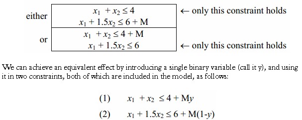
Now if y = 0 then only constraint (1) holds, and if y = 1 then only constraint (2) holds, exactly the kind of either/or behaviour we wanted. The downside, of course, is that a linear program has been converted to a mixed -integer program that is harder to solve.
k out of N Constraints Must Hold – This is a generalization of the either/or situation described above. For example, we may want any 3 out of 5 constraints to hold. This is handled by introducing N binary variables, y1…yN, one for each constraint, as follows:
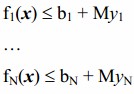
and including the following additional constraint:
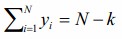
This final constraint works as follows: since we want k constraints to hold, there must be N – k constraints that don’t hold, so this constraint insures that N -k of the binary variables take the value 1 so that associated M values are turned on, thereby eliminating the constraint.
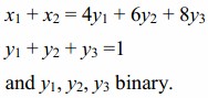
Functions Having N Discrete Values – Sometimes you have a resource that is available in only certain discrete sizes. For example, the metal finishing machine may be an equality that has 3 settings: x1 + x2 = 4 or 6 or 8. This can be handled by introducing one binary variable for each of the right hand side values. Where there are N discrete right hand sides, the model becomes:
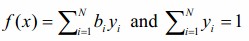
This assures that exactly one of the right hand side values is chosen. In the metal finishing machine example, the model would be:
Fixed Charges and Set -up Costs – Fixed charges or set-up costs are incurred when there is some kind of fixed initial cost associated with the use of any amount of a variable, even a tiny amount. For example, if you wish to use any amount at all of a new type of metal finishing for the ABC Company, then you incur a one -time set-up cost for buying and installing the required new equipment. Fixed charges and set-up costs occur frequently in practice, so it is important to be able to model them. Mathematically speaking, a set-up charge is modeled as follows:
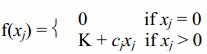
where K is the fixed charge. This says that there are no charges at all if the resource represented by xj is not used, but if it is used, then we incur both the fixed charge K and the usual charges associated with the use of xj, represented by cjxj.
The objective function must also be modified. It becomes:
minimize Z = f(xj) + (rest of objective function)
The minimization: set-up costs are only interesting in the cost -minimization context. If it is cost -maximization (a strange concept…) then we would of course always incur the set -up cost by insuring that every resource was always used.
The final model introduces a binary variable y that determines whether or not the set-up charge is incurred:
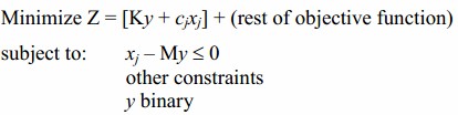
This behaves as follows. If xj > 0, then the first constraint insures that y = 1, so that the fixed charge in the objective function is properly applied. However, if xj = 0, then y could be 0 or 1: the first constraint is not restrictive enough in this sense. We want y to be zero in this case so that the set -up cost is not unfairly applied, and something in the model actually does influence y to be zero. Can you see what it is? It is the minimization objective. Given the free choice in this case between incurring a set-up cost or not, the minimization objective will obviously choose not to. Hence we have exactly the behaviour that we wish to model. Once again, though, we have converted a linear program to a mixed-integer linear program.
