Process Capability and Performance

Process capability is a predictable pattern of statistically stable behavior where the chance causes of variation are compared to the engineering specifications. A capable process is a process whose spread on the bell-shaped curve is narrower than the tolerance range.

Process Capability Studies

A process capability study attempts to quantify whether a process can consistently meet the standards set by internal or external customers. Since this study yields a prediction, and predictions should be made from relatively stable processes, a process capability study should only be used in a relatively controlled and stable process environment.

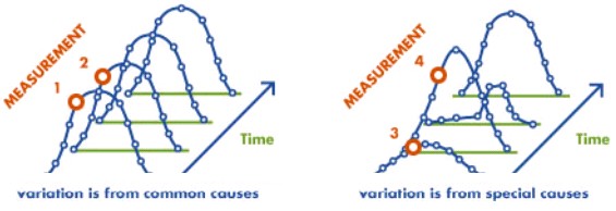
Measuring capability can be challenging because it is, by definition, a point estimate. Every process has unpredictable instability, which creates an inherent risk of estimate errors. Since there is no confidence interval related for mean and standard deviation, there is no confidence interval for capability, therefore risk cannot be quantified. The user must accept the risk of variability related to instability. If the variation is due to a common cause, the output will still form a distribution that is relatively stable as the variation is constant. In this case, a process capability study may be completed but, if the variation is a result of a special cause, then the output is not as stable and not as predictable. In this case, a process capability study may have problems with its accuracy.

The objective of a process capability study is to establish a state of control over the manufacturing process and then maintaining that state of control through time.

Study Procedure

It includes various steps, as

1. Select a process to study which is critical and can be selected using several techniques like a Pareto analysis or a cause-and-effect diagram.
2. Verify or define the process parameters. Verification of what the process entails, its boundaries, and gain agreement on the process’s definition. Many of these steps are completed when developing a process map.
3. Conduct a measurement systems analysis to ensure that the measurement methods produce sound data.
4. Select a process capability analysis method like Cpk, Cp, Ppk and Pp.
5. Obtain the data and conduct an analysis.
6. Develop an estimate of the process capability. This estimate can be compared to the standards set by internal or external customers.

After completing a process capability study, address any special causes of variation that can be isolated. If able, eliminate the special causes that are not desirable. In some cases, a special cause of variation may be desirable if it produces a better product or output. In that circumstance, if possible, attempt to make the special cause a common cause to ensure the benefit is achieved equally on all output.

Identifying Characteristics

Characteristics selected to be part of a process capability study should meet certain requirements, as

1. The characteristic should be important relative to the quality of the product or process. A process may have 15 characteristics, but only one or two should be selected for inclusion in the process capability study.
2. The characteristics are Ys or outcomes to process steps that meet customer requirements. The Ys are changed by changing the Xs or inputs.
3. The characteristic’s value should be adjustable.
4. The operating parameters that influence the characteristic should be able to be determined and controlled.
5. Sometimes, the characteristic selected has a history of being the most difficult item to control.

Identifying Specifications/Tolerances

The process specifications or tolerances are determined either by customer requirements, industry standards, or the organization’s engineering department.

Developing Sampling Plans

If the process fits a normal distribution and is in statistical control, then the standard deviation can be estimated from

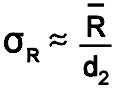
For new processes, for example for a project proposal, a pilot run may be used to estimate the process capability.

Specification Limits

Specification limits are set by the customer, and result from either customer requirements or industry standards. The amount of variance (process spread) the customer is willing to accept sets the specification limits. A customer wants a supplier to produce 12-inch rulers. Specifications call for an acceptable variation of +/- 0.03 inches on each side of the target (12.00 inches). The customer is saying acceptable rulers will be from 11.97 to 12.03 inches. If the process is not meeting the customer’s specification limits, two choices exist to correct the situation:

1. Change the process’s behavior.
2. Change the customer’s specification (requires customer approval).

Examples of Specification Limits – Specification limits are commonly found in

1. Blueprints
2. Engineering drawings and specs
3. Industry standards
4. Self-imposed standards within a shop
5. Federally mandated standards (e.g., emissions controls)

Verifying Stability and Normality 

If only common causes of variation are present in a process, then the output of the process forms a distribution that is stable over time and is predictable. If special causes of variation are present, the process output is not stable over time.

While the process is currently capable, stability may need to be improved to assure continued capability. Since the process is stable, but not capable, we can be reasonably sure the lack of capability is reasonably correct. The process must be improved to become capable. The lack of stability makes it difficult to estimate the level of capability with any certainty. First, we need to reduce variation and remove special causes of variation to improve stability so we will have reasonable estimates of the centering of the process. Following that, we may need to re-center the process and/or further reduce process variation.

Process performance vs. specification

The performance metric indices establish a controlled process, and then maintain that process over time. Numbered values are a shortcut method indicating the quality level of a process in parts per million (ppm). Once the status of the process is determined, the causes in variation (based on statistical significance) may be identified. Courses of action might be to

1. Do nothing.
2. Change the specifications.
3. Center the process.
4. Reduce the variation in the Six Sigma process spread.
5. Accept the losses.

Process Limits

A stable process can be monitored to determine if changes that occur are due to factors other than random variation. Such observation determines whether changes are necessary and if any corrective actions are required. Process limits are the voice of the process based on the variation of the products produced. The supplier collects data over time to determine the variation in the units against the customer’s specification. These data points collected over time establish the process curve.

Having a predictable process producing 100 percent conformances is the ideal state. Day-to-day control charts help identify assignable causes to any variations that occur. Control charts are special types of time series charts in which control limits are calculated around the central location, or mean, of the variable being plotted.

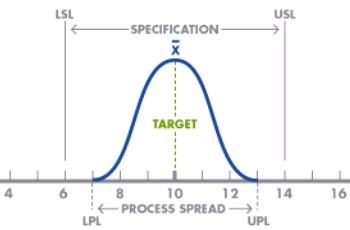
A process capability diagram displays both the voice of the process and the voice of the customer. To draw one of these diagrams

1. Locate the mean of the distribution (X) and draw a normal curve that reflects the upper and lower process limits (UPL, LPL) to the data.
2. Draw the customer specifications with the upper and lower limits for those specifications as appropriate (USL, LSL). Note that a customer may only have a lower limit or just an upper limit.

Process Performance Metric

It is a measure of an organization’s activities and performance and includes metrics like percentage defective which is defined as the (Total number of defective parts)/(Total number of parts) X 100. So if there are 1,000 parts and 10 of those are defective, the percentage of defective parts is (10/1000) X 100 = 1%. Other metrics have been discussed earlier and are summarized as

Performance Metric	Description
Percentage Defective	What percentage of parts contain one or more defects?
Parts per Million (PPM)	What is the average number of defective parts per million? This is the same figure in metric 1 above of “percentage defective” multiplied by 1,000,000.
Defects per Unit (DPU)	What is the average number of defects per unit?
Defects per Opportunity (DPO)	What is the average number of defects per opportunity? (where opportunity = number of different ways a defect can occur in a single part
Defects per million Opportunities (DPMO)	The same figure in metric 3 above of defects per opportunity multiplied by 1,000,000
Rolled throughput yield (RTY)	The yield stated as a percentage of the number of parts that go through a multi-stage process without a defect.
Process sigma	The sigma level associated with either the DPMO or PPM level found in metric 2 or 5 above.
Cost of poor quality	The cost of defects: either internal (rework/scrap) or external (warranty/product)

Process capability indices

Process capability indices includes Cp and Cpk, who identify the current state of the process and provide statistical evidence for comparing after-adjustment results to the starting point.

Cp – It measures the ratio between the specification tolerance (USL-LSL) and process spread. Whenever a process which is normally distributed and is exactly mid-way between the specification limits, would yield a Cp of 1 if the spread is +/- 3 standard deviations. The usual accepted minimum value for Cp is 1.33. It’s requirements for both an upper and lower specification and usage after the process is centered, is the major limitation. It is computed as

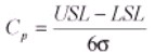
It is used to identify the process’s current state and measures the actual capability of a process to operate within customer defined specification limits hence, it should be used when the data set is from a controlled, continuous process. Hence, it needs standard deviation/Sigma information with USL and LSL specifications. Cp indicates the amount of variation in the process but not about the process’s ability to align with the target.

Cpk 

It measures the absolute distance of the mean to the nearest specification limit. Usually a Cpk value of minimum 1 and maximum 1.33 is desired. It needs the centering process similar as that for Cp. Along with Cp, Cpk provides a common measurement for assigning an initial process capability to center on specification limits. It is computed as

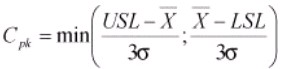
Cp measures “can it fit” while Cpk measures “does it fit.”. If Cp= Cpk , then the process is centered.

Cpm 

It is also referred to as the Taguchi index. It is more accurate and reliable than the other indices. It focuses on reducing the variation from a target value (T). Variation from the target T is expressed as process variability or σ2 and process centering (µ – T), where μ= process average. Cpm provides a common measurement assigning an initial process capability to a process for aligning the mean of the sample to the target. It is computed as

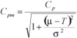
With T is the target value, μ is the expected value and σ is the standard deviation. It is applied if the target is not the center or mean of the USL – LSL or when establishing an initial process capability during the Measure phase. Higher Cpm value, indicates more likely the output of the process meet the specs and the target.

Sigma and Process Capability

When means and variances wander over time, a standard deviation (symbolized by the Greek letter σ) is the most common way to describe how data in a sample varies from its mean.

A Six Sigma goal is to have 99.99976% error-free work (reducing the defects to 3.4 per million). By computing sigma and relating to a process capability index such as Ppk, it can be determined the number of non-conformances (or failure rate) produced by the process. To compute sigma (σ), use the following equation for a population

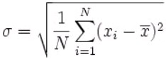
With, N is the number of items in the population, is the mean of the population data and x is each data point.

Process Performance Indices

The most used process performance indices are Pp, Ppk, and Cpm which depict the present status

of the process and also act as an important tool for improvement of the process. These metrics have a common purpose as process capability indices but, they differ in their approach.

Pp 

It measures the ratio between the specification tolerance and process spread. It helps to measure improvement over time as it signals where the process is in comparison to the customer’s specifications. It is computed as

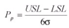
It is used for collecting continuous data and the process is not in control. It depicts the amount of variation, but not alignment to the target and for process to be in control, a process must only have common causes for each of the data points (no data points existing beyond the UCL or LCL).

Ppk 

It measures the absolute distance of the mean to the nearest specification limit. It provides an initial measurement to center on specification limits. It also examines variation within and between subgroups. It is computed as

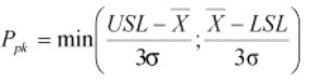
It is used with continuous data and the process is not in control. It indicates alignment to the USL and LSL but not the amount of variation.

Short-term vs. long-term capability

Short-term capability is measured over a very short time period since it focuses on the machine’s ability based on design and quality of construction. By focusing on one machine with one operator during one shift, it limits the influence of other outside long-term factors, including operator, environmental conditions such as temperature and humidity, machine wear and different material lots.

Thus, short-term capability can measure the machine’s ability to produce parts with a specific variability based on the customer’s requirements. Short-term capability uses a limited amount of data relative to a short time and the number of pieces produced to remove the effects of long-term components. If the machines are not capable of meeting the customer’s requirements, changes may have a limited impact on the machine’s ability to produce acceptable parts. Remember, though, that short-term capability only provides a snapshot of the situation. Since short-term data does not contain any special cause variation (such as that found in long-term data), short-term capability is typically rated higher.

When a process capability is determined using one operator on one shift, with one piece of equipment, the process variation is relatively small. Control limits based on a short-term process evaluation are closer together than control limits based on the long-term process.

A modified and R chart can be used for short runs, based on an initial 3 to 10 pieces, using a calculated value compared with a critical value. Inflated D₄ and A₂ values are used to establish control limits. Control limits are recalculated after additional groups are run.

The X and MR chart can also be used for small runs, with a limited amount of data. The X represents individual data values, and the MR is the moving range, a measure of piece to piece variability.

Process capability or Cpk values determined from either of these methods must be considered preliminary information. As the number of data points increases, the calculated process capability will approach the true capability.

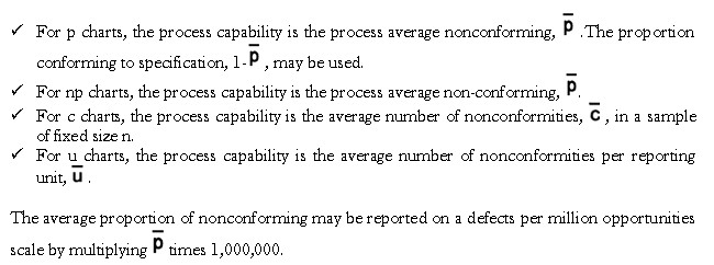
Process capability for attributes data

The control chart represents the process capability, once special causes have been identified and removed from the process. For attribute charts, capability is defined as the average proportion or rate of nonconforming product.