Probability Distributions

Distribution

Prediction and decision-making needs fitting data to distributions (like normal, binomial, or Poisson). A probability distribution identifies whether a value will occur within a given range or the probability that a value that is lesser or greater than x will occur or the probability that a value between x and y will occur.

A distribution is the amount of variation in the outputs of a process, expressed by shape (symmetry, skewness and kurtosis), average and standard deviation. Symmetrical distributions the mean represents the central tendency of the data but for skewed distributions, the median is the indicator. The standard deviation provides a measure of variation from the mean. Similarly skewness is a measure of the location of the mode relative to the mean thus, if mode is to the mean’s left then the skewness is negative else positive but for symmetrical distribution, skewness is zero. Kurtosis measures the peakness or relative flatness of the distribution and the kurtosis is higher for a higher and narrower peak.

Probability Distribution

It is a mathematical formula relating the values of a characteristic or attribute with their probability of occurrence in the population. It depicts the possible events and the associated probability for each of these events to occur. Probability distribution is divided as

1. Discrete data describe a finite set of possible occurrences for the data like rolling a dice with the random variable can take value from 1, 2, 3, 4, 5 or 6. The most used discrete probability distributions are the binomial, the Poisson, the geometric, and the hypergeometric distribution.
2. Continuous data describes a continuum of possible occurrences that is unbroken as, the distribution of body weight is a random variable with infinite number of possible data points.

Probability Density Function

Probability distributions for continuous variables use probability density functions (or PDF), which are mathematically model the probability density shown in a histogram but, discrete variables have probability mass function. PDFs employ integrals as the summation of area between two points when used in an equation. If a histogram shows the relative frequencies of a series of output ranges of a random variable, then the histogram also depicts the shape of the probability density for the random variable hence, the shape of the probability density function is also described as the shape of the distribution. An example illustrates it

Example: A fast-food chain advertises a burger weighing a quarter-kg but, it is not exactly 0.25 kg. One randomly selected burger might weigh 0.23 kg or 0.27 kg. What is the probability that a randomly selected burger weighs between 0.20 and 0.30 kg? That is, if we let X denote the weight of a randomly selected quarter-kg burger in kg, what is P(0.20 < X < 0.30)?

This problem is solved by using probability density function as, imagine randomly selecting, 100 burgers advertised to weigh a quarter-kg. If weighed the 100 burgers, and created a density histogram of the resulting weights, perhaps the histogram might be

.

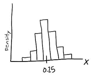
In this case, the histogram illustrates that most of the sampled burgers do indeed weigh close to 0.25 kg, but some are a bit more and some a bit less. Now, what if we decreased the length of the class interval on that density histogram then, it will be as

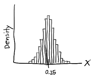
Now, if it is pushed further and the interval is decreased then, the intervals would eventually get small that we could represent the probability distribution of X, not as a density histogram, but rather as a curve (by connecting the “dots” at the tops of the tiny rectangles) as

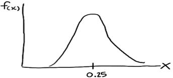
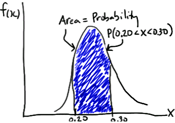
Such a curve is denoted f(x) and is called a (continuous) probability density function. A density histogram is defined so that the area of each rectangle equals the relative frequency of the corresponding class, and the area of the entire histogram equals 1. Thus, finding the probability that a continuous random variable X falls in some interval of values involves finding the area under the curve f(x) sandwiched by the endpoints of the interval. In the case of this example, the probability that a randomly selected burger weighs between 0.20 and 0.30 kg is then this area, as

Distributions Types

Various distributions are

1. Binomial – It is used in finite sampling problems when each observation has only one of two possible outcomes, such as pass/fail.
2. Poisson – It is used for situations when an attribute possibility is that each sample can have multiple defects or failures.
3. Normal – It is characterized by the traditional “bell-shaped” curve, the normal distribution is applied to many situations with continuous data that is roughly symmetrical around the mean.
4. Chi-square – It is used in many situations when an inference is drawn on a single variance or when testing for goodness of fit or independence. Examples of use of this distribution include determining the confidence interval for the standard deviation of a population or comparing the frequency of variables.
5. Student’s t – It is used in many situations when inferences are drawn without a variance known in the case of a single mean or the comparison of two means.
6. F – It is used in situations when inferences are drawn from two variances such as whether two population variances are different in magnitude.
7. Hypergeometric – It is the “true” distribution. It is used in a similar manner to the binomial distribution except that the sample size is larger relative to the population. This distribution should be considered whenever the sample size is larger than 10% of the population. The hypergeometric distribution is the appropriate probability model for selecting a random sample of n items from a population without replacement and is useful in the design of acceptance-sampling plans.
8. Bivariate – It is created with the joint frequency distributions of modeled variables.
9. Exponential – It is used for instances of examining the time between failures.
10. Lognormal – It is used when raw data is skewed and the log of the data follows a normal distribution. This distribution is often used for understanding failure rates or repair times.
11. Weibull – It is used when modeling failure rates particularly when the response of interest is percent of failures as a function of usage (time).

Binomial Distribution

It is used to model discrete data having only two possible outcomes like pass or fail, yes or no and which are exactly two mutually exclusive outcomes. It can tell you about the occurrence of an event, but not about the event’s magnitude. Events in these distributions are independent of each other.

It may be used to find the proportion of defective units produced by a process and used when population is large – when N> 50 with small size of sample compared to the population. The ideal situation is when sample size (n) is less than 10% of the population (N) or n< 0.1N. The binomial distribution is useful to find the number of defective products if the product either passes or fails a given test. The mean, variance, and standard deviation for a binomial distribution are µ = np, σ2= npq and σ =√npq. The essential conditions for a random variable are fixed number of observations (n) which are independent of each other, every trial results in either of the two possible outcomes and if the probability of a success is p and the probability of a failure is 1 -p.

Binomial distribution can be applied as

1. count the number of defective or non-defective items in a sample
2. investigate the process yield
3. sample for attributes – for instance, using acceptance sampling

The binomial distribution mean is calculated as n multiplied by p. In other words, it’s a function of the number or sample size multiplied by the rate of the event in the population. This tells you how many of your samples in a population are likely to exhibit the issue or the defect. Standard deviation is calculated as the square root of [np (1 – p)]. This is useful for understanding the range of the sigma value in a population of data.

The binomial probability distribution equation will show the probability p (the probability of defective) of getting x defectives (number of defectives or occurrences) in a sample of n units (or sample size) as

As an example if a product with a 1% defect rate, is tested with ten sample units from the process, Thus, n= 10, x= 0 and p= .01 then, the probability that there will be 0 defective products is

Poisson Distribution

It estimates the number of instances a condition of interest occurs in a process or population. It focuses on the probability for a number of events occurring over some interval or continuum where µ, the average of such an event occurring, is known like project team may want to know the probability of finding a defective part on a manufactured circuit board. Most frequently, this distribution is used when the condition may occur multiple times in one sample unit and user is interested in knowing the number of individual characteristics found like critical attribute of a manufactured part is measured in a random sampling of the production process with non-conforming conditions being recorded for each sample. The collective number of failures from the sampling may be modeled using the Poisson distribution. It can also be used to project the number of accidents for the following year and their probable locations. The essential condition for a random variable to follow Poisson distribution is that counts are independent of each other and the probability that a count occurs in an interval is the same for all intervals. The mean and the variance of the Poisson distribution are the same, and the standard deviation is the square root of the mean hence, µ = σ2 and σ =√µ =√σ2.

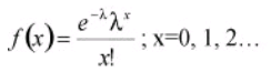
The Poisson distribution can be an approximation to the binomial when p is equal to or less than 0.1, and the sample size n is fairly large (generally, n >= 16) by using np as the mean of the Poisson distribution. Considering f(x) as the probability of x occurrences in the sample/interval, λ as the mean number of counts in an interval (where λ > 0), x as the number of defects/counts in the sample/interval and e as a constant approximately equal to 2.71828 then the equation for the Poisson distribution is as

Normal Distribution

A distribution is said to be normal when most of the observations are clustered around the mean. It charts a data set of which most of the data points are concentrated around the average (mean) in a symmetrical manner, thus forming a bell-shaped curve. The normal distribution’s shape is unique in that the most frequently occurring value is in the middle of the range and other probabilities tail off symmetrically in both directions.

The mean is the central value and is represented by the U shape in the curve. The sigma value is represented by a sigma symbol. A normal distribution has a unimodal shape, meaning it has a single peak. It also has symmetrical distribution around the mean. Often the mean, median, and mode are the same in the data of the distribution. The higher the sigma value, the flatter, or more shallow, the curve. For example, if three normal distributions have the same mean but standard deviations, respectively, of 0.7, 1, and 1.5, the distribution with the sigma value of 1.5 will be the flattest.

The normal distribution is used for continuous (measurement) data that is symmetric about the mean. The graph of the normal distribution depends on the mean and the variance. When the variance is large, the curve is short and wide and when the variance is small, the curve is tall and narrow.

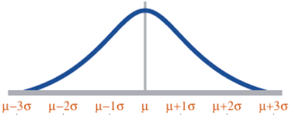
The normal distribution is also called as the Gaussian or standard bell distribution. The population mean μ is zero and that the population variance σ2 equals one as in the figure and σ is the standard deviation. The normal probability density function is

For normal distribution, the area under the curve lies between µ − σ and µ + σ.

Z- transformation

The shape of the normal distribution depends on two factors, the mean and the standard deviation. Every combination of µ and σ represent a unique shape of a normal distribution. Based on the mean and the standard deviation, the complexity involved in the normal distribution can be simplified and it can be converted into the simpler z-distribution. This process leads to the standardized normal distribution, Z = (X − µ)/σ. Because of the complexity of the normal distribution, the standardized normal distribution is often used instead.

Chi-Square Distribution

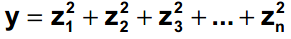
The chi-square (χ2) distribution is used when testing a population variance against a known or assumed value of the population variance. It is skewed to the right or with a long tail toward the large values of the distribution. The overall shape of the distribution will depend on the number of degrees of freedom in a given problem. The degrees of freedom are 1 less than the sample size. It is formed by adding the squares of standard normal random variables. For example, if z is a standard normal random variable, then the following is a chi-square random variable (statistic) with n degrees of freedom

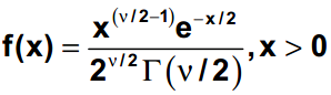
The chi-square probability density function where v is the degree of freedom and (x) is the gamma function is

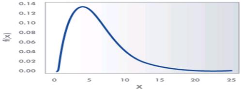
An example of a χ2 distribution with 6 degrees of freedom is as

Student t Distribution

It was developed by W.S. Gosset. The t distribution is used to determine the confidence interval of the population mean and confidence statistics when comparing the means of sample populations but, the degrees of freedom for the problem must be known n. The degrees of freedom are 1 less than the sample size.

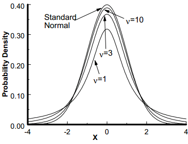
The student’s t distribution is a symmetrical continuous distribution and similar to the normal distribution, but the extreme tail probabilities are larger than for the normal distribution for sample sizes of less than 31. The shape and area of the t distribution approaches towards the normal distribution as the sample size increases. The t distribution can be used whenever samples are drawn from populations possessing a normal, bell-shaped distribution. There is a family of curves, one for each sample size from n =2 to n = 31.

F Distribution

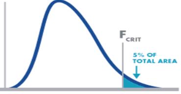
The F distribution or F-test is a tool used for assessing the ratio of independent variances or equality of variances from two normal populations. It is used in the Analysis of Variance (ANOVA, a technique frequently used in the Design of Experiments to test for significant differences in variance within and between test runs).

If U and V are the variances of independent random samples of size n and m taken from normally distributed populations with variances of w and z, then

which is a random variable with an F distribution with v1 = n-1 and v2 = m – 1. The F-distribution is represented by

with (s1)2 is the variance of the first sample (n1- 1 degrees of freedom in the numerator) and (s2)2 is the variance of the second sample (n2- 1 degrees of freedom in the denominator), given two random samples drawn from a normal distribution.

The shape of the F distribution is non-symmetrical and will depend on the number of degrees of freedom associated with (s1)2 and (s2)2. The distribution for the ratio of sample variances is skewed to the right (the large values).

Geometric distribution

It addresses the number of trials necessary before the first success. If the trials are repeated k times until the first success, we would have k−1 failures. If p is the probability for a success and q the probability for a failure, the probability of the first success to occur at the kth trial is P(k, p) = p(q)k−1 with the mean and standard deviation are µ =1/p and σ = √q/p.

Hypergeometric Distribution

The hypergeometric distribution applies when the sample (n) is a relatively large proportion of the population (n >0.1N). The hypergeometric distribution is used when items are drawn from a population without replacement. That is, the items are not returned to the population before the next item is drawn out. The items must fall into one of two categories, such as good/bad or conforming/nonconforming.

The hypergeometric distribution is similar in nature to the binomial distribution, except the sample size is large compared to the population. The hypergeometric distribution determines the probability of exactly x number of defects when n items are samples from a population of N items containing D defects. The equation is

With, x is the number of nonconforming units in the sample (r is sometimes used here if dealing with occurrences), D is the number of nonconforming units in the population, N is the finite population size and n is the sample size.

Bivariate Distribution

When two variables are distributed jointly the resulting distribution is a bivariate distribution. Bivariate distributions may be used with either discrete or continuous data. The variables may be completely independent or a covariance may exist between them.

The bivariate normal distribution is a commonly used version of the bivariate distribution which may be used when there are two random variables. This equation was developed by Freund in 1962 as

With

1. -∞ < x < ∞
2. -∞ < y < ∞
3. -∞ < μ1< ∞
4. -∞ < μ2< ∞
5. σx> 0, σx> 0
6. μ1 and μ2 are the two population means
7. First σ2 and second σ2 are the two variances
8. ρ is the correlation coefficient of the random variables

Exponential Distribution

It is used to analyze reliability, and to model items with a constant failure rate. The exponential distribution is related to the Poisson distribution and used to determine the average time between failures or average time between a numbers of occurrences. The mean and the standard deviation are µ =1/λ and σ =1/λ.

For example, if there is an average of 0.50 failures per hour (discrete data – Poisson distribution), then the mean time between failure (MTBF) is 1 / 0.50 = 2 hours (continuous data – exponential distribution). If a random variable x is distributed exponentially, then its reciprocal y =1/x follows a Poisson distribution. The opposite is also true. If x follows a Poisson distribution, then the reciprocal y = 1/x is exponentially distributed. The exponential distribution equation is

With μ is the mean (also sometimes referred to as θ), λ is the failure rate which is the same as1/μ and x is the x-axis values. When this equation is integrated, it results in cumulative probabilities as

Lognormal Distribution

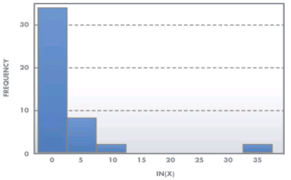
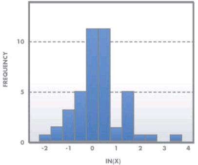
The most common transformation is made by taking the natural logarithm, but any base logarithm, such as base 10 or base 2 may be used. It is used to model various situations such as response time, time-to-failure data, and time-to-repair data. Lognormal distribution is a skewed-right distribution (with most data in the left tail), and consists of the distribution of the random variable whose logarithm follows the normal distribution.

The lognormal distribution assumes only positive values. When the data follows a lognormal distribution, a transformation of data can be done to make the data follow a normal distribution. Then probabilities, confidence intervals and tests of hypothesis can be conducted (if the data follows a normal distribution). The lognormal probability density function is

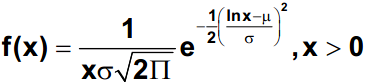
With μ is the location parameter or log mean and σ is the scale (or shape) parameter or standard deviation of natural logarithms of the individual values.

Weibull Distribution

The Weibull distribution is a widely used distribution for understanding reliability and is similar in appearance to the lognormal. It can be used to measure time to fail, time to repair, and material strength. The shape and dispersion of the Weibull distribution depends on two parameters β which is the shape parameter and θ which is the scale parameter but, both parameters are greater than zero.

The Weibull distribution is one of the most widely used distributions in reliability and statistical applications. The two and three parameter Weibull common versions. The difference is the three parameter Weibull distribution has a location parameter when there is some non-zero time to first failure. In general, the probabilities from a Weibull distribution can be found from the cumulative Weibull function as

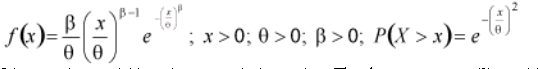
With, X is a random variable, x is an actual observation. The shape parameter (β) provides the Weibull distribution with its flexibility as

1. If β = 1, the Weibull distribution is identical to the exponential distribution.
2. If β = 2, the Weibull distribution is identical to the Rayleigh distribution.
3. If 3 < β < 4, then the Weibull distribution approximates a normal distribution.