Formatting data automatically
Formatting data with auto format
The steps to auto format are
- Select the range you want to format.
- On the Format menu, click AutoFormat.
- Click the format you want.
Format data with other option
With the help of this option we can customize which specific part of auto format should be applied i.e. whether auto formatting of font type, font size, pattern, border, etc. should be applied on to the selection or not. In MS-EXCEL 2003, it is available as ‘Options’ in the Auto Format dialog box.
Repeat Auto formatting
Auto formatting can be repeated to another range of cells, by again applying the steps given for formatting data with auto format, as above.
Copying formats to other cells
Copy a format with the format painter button
The steps to copy the format are
- Select a cell or range that has the formatting to copy.
- On the Formatting toolbar, click Format Painter.
- Select the cell or range to copy the formatting to.
Format from Toolbar
Excel primarily supports Textual and Numerical data. Formatting toolbar is used to format the data in Excel. The text formatting buttons and their usage are same as MS-Word together with some special buttons. The Formatting Toolbar in Excel is as under.

Following are the icons on the Formatting Toolbar
- Merge and Center
 : This option is useful for centering a label across several columns. In order to merge a label within multiple columns, enter the label in the first cell and then select all the cells across which the label is to be centered. Now choose Cells from Format menu select Alignment control tab and turn on the option Merge cells. In the end select Horizontal Alignment as Center.
  Currency Button : This option is used to put the currency symbol as prefix to the number type of data within selection. For changing the currency symbol, select Start menu and choose Settings. Click on the Control Panel option and use Regional Settings. Append the default currency symbol accordingly.
 Percentage Button: It allows the user to use percentage sign as suffix with the numeric data and multiply the number by 100 (hundred).
 Comma Button: It allows using comma separator after each three digits and decimal places for number type of data within selection. The subsequent buttons are used to increase or decrease number of decimal places. Normally it is used to round off the figures.
 Indent Buttons: These Indent buttons are used to change indentation within cell(s).
 Alter Indents: These buttons are used to alter the indentation within the cell.
 Border Buttons: It helps to give printable borders to the selected cell(s).
 Fill Color : This button helps to fill background of the selected cell(s).
 Font Color: This button helps to change the color of the selected text/number.
Format Dialog Box
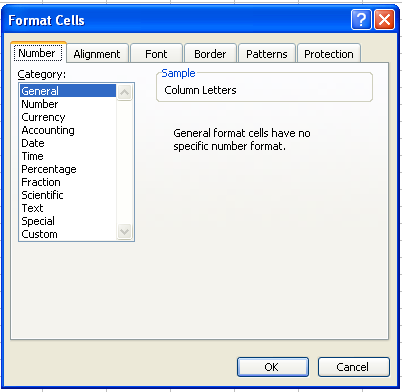
To format data in worksheet Excel supports several options. To apply such formats, select the Format menu and choose Cells from the list or press Ctrl + 1, the following dialog box for Formatting Cells will appear on your screen.
There following are the types of formatting that excel supports
Number Formats
The following options will be available to the user for applying any amount of formatting by selecting Number control tab and choosing from the given options.
- General: The default format of number will be applied under this option. Primarily it is used to remove or cancel any number format from the selection.
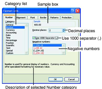
- Number: This type of formatting allows you to set number of decimal places, a thousands separator, and formatting of negative numbers.
- Currency: Under this option numbers are preceded with a default Currency sign immediately. You can also set here number of decimal places and the formatting of the negative numbers. Zero values will be displayed as well.
- Accounting: Under this option Currency sign and decimal places can set with the numbers. But the setting of Currency symbol with number is different from Currency format.
- Date: This option provides a variety of Date formats.
- Time: This option provides Different time formats.
- Percentage: This formatting suffixes a percentage sign with the number and multiply the number by 100 (hundred).
- Fraction: This option includes formats based on either the number of digits to display in the divisor (1, 2, or 3) or the fractional unit (halves, quarters, tenths, and so on).
- Scientific: Under this option numbers are displayed in scientific notation. For example 1.23E+01.
- Text: This option is used to change a number to text without adding other formatting. This is useful for numeric labels that may include leading zeros. The Text format must be applied before entering the cell’s contents, since the numbers entered and later formatted, as Text will always be treated as numbers.
- Special: This option is applicable for those having some special formats and is usually used for Telephone numbers, Zip Codes etc.
- Custom: This option provides a list of custom formats for numbers, dates, and times that you can select from or add to. You need to declare a pattern/format for this type of data for a group of cells. Before entering data, apply the formats first to get desired effects. Here the user can manipulate zero positions.
Changing Number format
We can use number formats to change the appearance of numbers, including dates and times, without changing the number behind the appearance. For example 23455 can be displayed in currency format as $23,455.00 whereas in percentage number format it will be 2345500%. The General format is the default number format. For the most part, what you enter in a cell that is formatted with the General format is what is displayed. However, if the cell is not wide enough to show the entire number, the General format rounds numbers with decimals and uses scientific notation for large numbers. For changing the number formats, we can use the formatting toolbar.
Following steps are to be taken for changing the number format
- Select the cells you want to format.
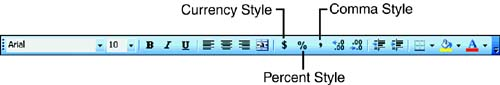
- Click Comma Style, (It applies the Comma style to the selected cells.) or Currency Style, or Percent Style on the Formatting toolbar, as shown in the figure below
Changing the date format
Following steps are to be taken for changing the date format
- Select the cells you want to format.
- On the Format menu, click Cells, and then click the Number tab.
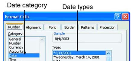
- In the Category list, click Date, and then click the format you want to use.
Days, months, and years To display days, months, and years, include the following format codes in a section. If you use “m” immediately after the “h” or “hh” code or immediately before the “ss” code, Microsoft Excel displays minutes instead of the month. To illustrate the details
| To display | Use this code |
| Months as 1–12 | M |
| Months as 01–12 | Mm |
| Months as Jan–Dec | Mmm |
| Months as January–December | Mmmm |
| Months as the first letter of the month | Mmmmm |
| Days as 1–31 | D |
| Days as 01–31 | Dd |
| Days as Sun–Sat | Ddd |
| Days as Sunday–Saturday | Dddd |
| Years as 00–99 | Yy |
| Years as 1900–9999 | Yyyy |
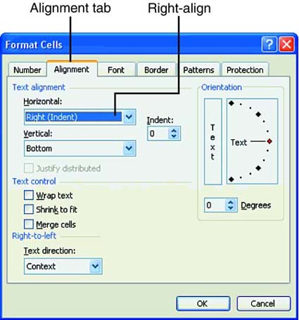
Changing Alignment
The alignment of any of the cell entry can be changed, as we require it. To change the alignment of the cell click Format on the menu bar, click on Cells option then select the Alignment tab, select the horizontal and the vertical alignment that is required. In Excel there are 9 type of alignment that can be done.
| Horizontal Alignment Options | |
| Alignment | What It Does |
| General | Aligns numbers and dates with the right side of the cell and text with the left side. |
| Left (Indent) | Aligns selected data with the left side of the cell. |
| Center | Centers data within the cell. |
| Right (Indent) | Aligns selected data with the right side of the cell. |
| Fill | Repeats the data to fill the entire width of the cell. |
| Justify | Aligns text with the right and left side of the cell. Use with the Wrap Text option in the Text Control section on the Alignment tab. |
| Center Across Selection | Centers a title or other text inside a range of cells, such as over columns. |
| Distributed (Indent) | Aligns text with the right and left side or top and bottom of the cell. Use with the Wrap Text option in the Text Control section on the Alignment tab. |
The Vertical alignment options specify how you want the text aligned in relation to the top and bottom of the cell(s).
Wrap Text
Word provides with the Wrap Text feature which allows text expansion for more than one line within a cell without changing the cell width, but cell height changes accordingly.
Shrink to Fit
This option adjusts the lengthy texts within a cell without changing the cell width as well as the cell height; only the text size will be reduced proportionately.
Merge Cells
This option allows the user to combine more than one cell to a single cell and also to break a merged cell into several numbers of cells. This option works only horizontally.
Orientation
This option facilitates the rotation of text or number within cell in any degree of angle within the limits. By clicking and dragging the red dot you can angle the data within cell. As you drag the red dot, the degrees of the angle are displayed in the Degrees box. You can also insert the value for degrees of angle within this Degrees text box.
Formatting Font
Style is a collection of formats such as font size, patterns, and alignment that you can define and save as a group. Hence, changing character styles means changing the font size or font style. It can be done through the buttons on the formatting toolbar, as shown in the figure
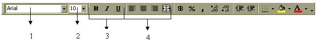
- To change Font Style
- To change Font Size
- To change Font Effects
- To change Text Alignment
The option of Font control tab facilitates to change the data appearance. The dialog box has all formatting options. The use of Font control tab is same as MS-Word. The Font Face, Size, Style, Color, Underline Style and other Effects, like Strikethrough, Superscript and Subscript can be amended using Format cells in MS-Excel.
Fill & Cell Borders
Following steps are to be taken to add borders –
- Select the cells you want to add borders to.
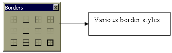
- To apply the most recently selected border style, click Borders on the Formatting toolbar.
To apply a different border style, click the arrow next to Borders, and then click a border on the palette. More border settings To apply additional border styles, click Cells on the Format menu, and then click the Border tab. Click the line style you want, and then click a button to indicate the border placement. To change the line style of an existing border, select the cells that the border appears on. On the Border tab, click a new style in the Style list, and then click the border you want to change in the diagram under Border. As displayed in the figure below
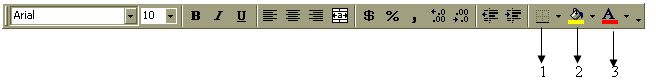
- To apply borders
- To change Fill color
- To change Font color
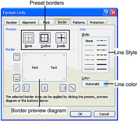
Cell Border dialog box
Removing cell gridlines
Following steps are to be taken to removing the cell gridlines
- Select the sheets on which you want to hide the gridlines.
- On the Tools menu, click Options, and then click the View tab.
- Under Window options, clear the Gridlines check box.
Customizing default currency – Changing $ to Rs.
Custom currency formats are saved with the workbook. To have Microsoft Excel always use a specific currency symbol, change the currency symbol selected in Regional Settings in Control Panel before starting MS-Excel.
Changing font for entire worksheet
For selecting entire worksheet either press Control + A or Click the Select All button present at the intersection of row and column header. Then change the font by the font box on the formatting toolbar.
Changing font for entire workbook
For selecting entire worksheet by right-clicking a sheet tab, and then click Select All Sheets on the shortcut menu. Then change the font by the font box on the formatting toolbar.
Conditional Formatting
MS-Excel provides the feature of Conditional Formatting used to apply format to selected cells based on predefined conditions. Conditional formatting is not a database feature, but it can be used to highlight most important data from a database. The font attributes, borders, or patterns can be applied to cells. For applying Conditional Formatting to a selection, choose Conditional Formatting from the Format menu, the following dialog box will appear on your screen.
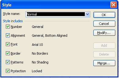
- Style name: Type a new style name in this box, turn on/off the Attributes accordingly and then click Add button.
- Modify: Click on Modify button to add or modify formatting decisions and call Cells formatting dialog box.
- Delete: This option is used to remove any existing style, which is done by selecting the style from the Style list and clicking on Delete button.
- Merge: This option is used to Import styles from another existing workbook. You must ensure to keep the source workbook open simultaneously. To apply a style, select the style name from the Style list and click OK.
Changing cell size
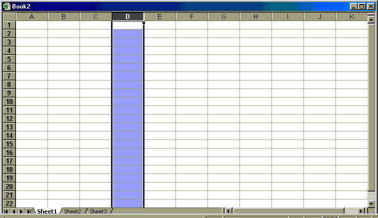
Changing Column Width
Column width can be changed by selecting the column and dragging till the desired width is not reached.
We may wish to make some entries that are longer than the default width of the cell i.e. 8 characters. Therefore, to adjust the entry into the cell width we need to increase the cell with that can be done by click Format on the menu bar, click on the Column option and select the width an small window appears asking we the width of the cell would appear, give the cell width to which we have to increase the width and click OK button. To fit the entry such that the Excel automatically adjusts the cell widths as per the entry select AutoFit Selection from the Format Þ Column in the menu bar
The size or width of a column controls how much information can be displayed in a cell. A text entry that is larger than the column width will be fully displayed only if the cells to the right are blank. If the cells to the right contain data, the text is interrupted. On the other hand, when numbers are entered in a cell, the column width is automatically increased to fully display the entry.
The default column width setting in Excel is 8.43. The number represents the average number of digits that can be displayed in a cell using the standard font. The column width can be any number from 1 to 255. When the worksheet is printed, it appears as it is does currently on the screen.
Therefore, we want to increase the column width to display the largest entry. Likewise, we can decrease the column width when the entries in a column are short As the figure below shows “D” column is selected for changing the width
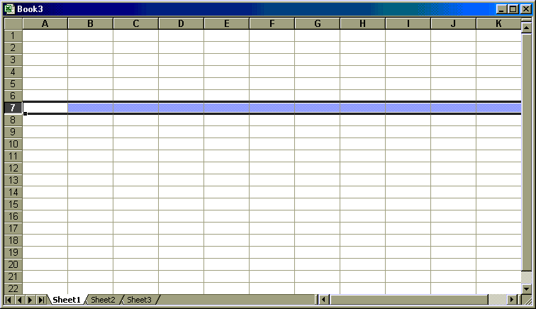
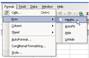
Changing Row Height
Row height can be changed by selecting the specific row and dragging till the desired height is not reached. As the figure below shows “7” row is selected for changing the height
We may wish to make some entries such that their height is more the default height. Therefore, to adjust the entry into the cell row height needs to increased this can be done by click Format on the menu bar, click on the Row option and select the Height a small window opens asking we the height of the row would appear, give the row height to which we have to increase the height and click OK button. To fit the entry such that the Excel automatically adjusts the cell width as per the entry, select AutoFit from the Format ÞRow in the menu bar
Row Height
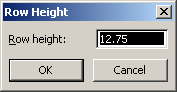
Value box
