A selection consisting of two or more cells is a range. The cells in a range can be adjacent or non-adjacent. An adjacent range is a rectangular block of adjoining cells. In the example shown below, the shaded areas show valid and invalid adjacent ranges. A non-adjacent range is two or more selected cells or ranges that are not adjoining.
To select an adjacent range, drag the mouse from one corner of the range to another. If the range is large, it is often easier to select the range by clicking on the first cell of the range, then hold down shift while clicking on the last cell of the range. We can quickly select an entire column or row by clicking the column or row letter or number. Dragging across the row or column heading selects adjacent rows and columns. To selects the non-adjacent cells or cell ranges, after selecting the first cell or range hold down (Ctrl) while selecting the rows or columns.
Creating Names
Rules for naming ranges, cells and formulas
Following rules are applicable for giving names to ranges, cells and formulas
- The first character of a name must be a letter or an underscore character. Remaining characters in the name can be letters, numbers, periods, and underscore characters.
- Names cannot be the same as a cell reference, such as Z$100 or R1C1.
- Yes, but spaces are not allowed. Underscore characters and periods may be used as word separators — for example, Sales_Tax or First.Quarter.
- A name can contain up to 255 characters.
- If a name defined for a range contains more than 253 characters, we cannot select it from the Name box.
- Names can contain uppercase and lowercase letters. Microsoft Excel does not distinguish between uppercase and lowercase characters in names. For example, if we have created the name Sales and then create another name called SALES in the same workbook, the second name will replace the first one.
Create Range Names
Following steps are to be taken to create range names
- Select the cell, range of cells that we want to name.
- Click the Name box at the left end of the formula bar.
- Type the name for the cells.
- Press ENTER.
Names can also be created as, when we select cells in labeled ranges to create formulas, Microsoft Excel can insert the labels in place of cell references in our formulas. Using labels can make it easier to see how a formula is constructed. We can use the Label Ranges dialog box (Insert menu, Name submenu, Label command) to specify the ranges that contain column and row labels on our worksheet.
Creating default range names
A reference identifies a cell or a range of cells on a worksheet and tells Microsoft Excel where to look for the values or data we want to use in a formula. With references, we can use data contained in different parts of a worksheet in one formula or use the value from one cell in several formulas. We can also refer to cells on other sheets in the same workbook, to other workbooks, and to data in other programs. References to cells in other workbooks are called external references. References to data in other programs are called remote references.
The A1 reference style, which refers to columns with letters (A through IV, for a total of 256 columns) and refers to rows with, numbers (1 through 65536). These letters and numbers are called row and column headings. To refer to a cell, enter the column letter followed by the row number. For example, D50 refers to the cell at the intersection of column D and row 50. To refer to a range of cells, enter the reference for the cell in the upper-left corner of the range, a colon (:), and then the reference to the cell in the lower-right corner of the range.
The R1C1 reference style uses a reference style where both the rows and the columns on the worksheet are numbered. The R1C1 reference style is useful for computing row and column positions in macros. In the R1C1 style, Excel indicates the location of a cell with an “R” followed by a row number and a “C” followed by a column number.
Saving Range Names
As discussed earlier, the name ranges created earlier are automatically saved.
Editing names
Steps to edit a name
Following steps are to be taken to Editing a name
- On the Insert menu, point to Name, and then click Define.
- In the Names in workbook box, click the name whose cell reference, formula, or constant we want to change.
- In the Refers to box, change the reference, formula, or constant.
Going to ranges
Select ranges using the name box
In the Name box, select the range. The name box, is a box at the left end of the formula bar that identifies the selected cell, chart item, or drawing object. Type the name in the Name box, and then press ENTER to quickly name a selected cell or range. To move to and select a previously named cell, click its name in the Name box.
Select ranges using the F5 key
F5 key opens the Go To dialog box or on the Edit menu, click Go To. In the Reference box, type the cell reference for the cell or range of cells. Microsoft Excel keeps track of the ranges we select by using the Name box or the Go To command. To return to a previous selection, click Go To on the Edit menu, and then double-click the cell reference in the Go to box.
Using names in formulas
You can use the labels of columns and rows on a worksheet to refer to the cells within those columns and rows. Or you can create descriptive names to represent cells, ranges of cells, formulas, or constant values. Labels can be used in formulas that refer to data on the same worksheet; if you want to represent a range on another worksheet, use a name.
A defined name in a formula can make it easier to understand the purpose of the formula. For example, the formula =SUM(FirstQuarterSales) might be easier to identify than =SUM(C20:C30).
Names are available to any sheet. For example, if the name ProjectedSales refers to the range A20:A30 on the first worksheet in a workbook, you can use the name ProjectedSales on any other sheet in the same workbook to refer to range A20:A30 on the first worksheet.
Names can also be used to represent formulas or values that do not change (constants). For example, you can use the name SalesTax to represent the sales tax amount (such as 6.2 percent) applied to sales transactions.
You can also link to a defined name in another workbook, or define a name that refers to cells in another workbook.
For example, the formula =SUM(Sales.xls!ProjectedSales) refers to the named range ProjectedSales in the workbook named Sales By default, names use absolute cell references.
Guidelines for names
- The first character of a name must be a letter or an underscore character. Remaining characters in the name can be letters, numbers, periods, and underscore characters.
- Names cannot be the same as a cell reference, such as Z$100 or R1C1.
- More than one word be used but spaces are not allowed. Underscore characters and periods may be used as word separators— for example, Sales_Tax or First.Quarter.
- A name can contain up to 255 characters.
Names can contain uppercase and lowercase letters. Microsoft Excel does not distinguish between uppercase and lowercase characters in names. For example, if you have created the name Sales and then create another name called SALES in the same workbook, the second name will replace the first one.
Cell Referencing
Copying formulas
When we copy a formula, absolute cell references do not change; relative cell references will change. The steps to move a formula are
- Select the cell that contains the formula we want to copy.
- Point to the border of the selection.
- To copy the cell, hold down CTRL as we drag.
- We can also copy formulas into adjacent cells by using the fill handle. (Fill handle is the small black square in the corner of the selection. When we point to the fill handle, the pointer changes to a black cross. To copy contents to adjacent cells or to fill in a series such as dates, drag the fill handle. To display a shortcut menu that contains fill options, hold down the right mouse button as we drag the fill handle.)
- Select the cell that contains the formula, and then drag the fill handle over the range we want to fill.
Relative Reference
A relative reference is a cell or range reference in a formula whose location is interpreted by Excel in relation to the position of the cell that contains the formula. The relative relationship between the referenced cell and the new location is maintained. Because relative references automatically adjust for the new location, the relationship between cells in both the copied and pasted formula is the same although the cell references are different. It can also be defined as, a cell reference, such as A1, that’s used in a formula, which changes when the formula is copied to another cell or range. After the formula is copied and pasted, the relative reference in the new formula is changed to refer to a different cell that is the same number of rows and columns away from the formula as the original relative cell reference is to the original formula. For example, if cell A3 contains the formula =A1+A2 and we copy cell A3 to cell B3, the formula in cell B3 becomes =B1+B2.
Absolute Reference
An absolute reference is a cell or range reference in a formula whose location does not change when the formula is copied. To stop the relative adjustment of cell references, enter a $ (dollar sign) character before the column letter and row number. This changes the cell reference to absolute. When a formula containing an absolute cell reference is copied to another row and column location in the worksheet, the cell reference does not change. It is an exact duplicate of the cell reference in the original formula.
A cell reference can also be a mixed reference. In this type of reference, either the column letter or the row number is preceded with the $ sign. This makes only the row or column absolute changes relative
to its new location in the worksheet. It can also be defined as, that in a formula, the exact address of a cell, regardless of the position of the cell that contains the formula. An absolute cell reference takes the form $A$1, $B$1, and so on. Some cell references are mixed. An absolute row reference takes the form A$1, B$1 and so on. An absolute column reference takes the form $A1, $B1, and so on. Unlike relative references, absolute references don’t automatically adjust when we copy formulas across rows and down columns.
| Contents of G8 | Type of Reference |
| $G$8 | Absolute reference |
| G$8 | Mixed reference |
| $G8 | Mixed reference |
| G8 | Relative reference |
Referencing Multiple Sheets.
To reference data in another sheet in the same workbook, we enter a formula that references cells in other worksheets. A formula tat contains references to cells in other sheets of a workbook allows we to use data from multiple sheets and to calculate new values based on this data. The formula contains a sheet reference consisting of the name of the sheet, followed by an exclamation point and the cell of the current sheet. A formula can be created using references on multiple sheets; for example =sheet! A1+sheet2!b2. If the sheet name contains non-alphabetic characters, such as a space, the sheet name (or path) must be enclosed in single quotation marks.
The link can also be created by entering a 3-D reference in a formula, a 3-D reference to the same cell or range on multiple sheets in the same workbook. A 3-d reference consists of the names of the beginning and ending sheets enclosed in quotes and separated by a colon. This is followed by an exclamation point and the cell or range reference. The cell or range reference is the same on each sheet in the specified sheet range.
| 3- D reference | Description |
| =Sum (sheet1: sheet! h6:k6) | Sums the values in cells H6 through K6 in sheets 1,2,3,4 |
| =Sum (sheet1! H6:H6) | Sums the values in cells H6 through K6 in sheet 1 |
| =Sum (Sheet1: Sheet4! H6) | Sums the values in cell H6 of sheets 1,2,3,4 |
Moving formulas
When we move a formula, the cell references within the formula do not change. The steps to move a formula are –
- Select the cell that contains the formula you want to move.
- Point to the border of the selection.
- To move the cell, drag the selection to the upper-left cell of the paste area. Microsoft Excel replaces any existing data in the paste area.
What are Functions?
As we had already discussed earlier, functions are predefined formulas that perform calculations by using specific values, called arguments, in a particular order, or structure. For example, the SUM function adds values or ranges of cells, and the PMT function calculates the loan payments based on an interest rate, the length of the loan, and the principal amount of the loan.
Category of functions
- Mathematical Functions
- Statistical Functions
- Financial Functions
- Date and Time Functions
- Logical Functions
- String Functions
- Database and List Management Functions
- Lookup & Reference
Applying functions
The ROUND Function
Rounds a number to a specified number of digits.
ROUND (number, num_digits)
Number is the number we want to round.
Num_digits specifies the number of digits to which we want to round number.
- If num_digits is greater than 0 (zero), then number is rounded to the specified number of decimal places.
- If num_digits is 0, then number is rounded to the nearest integer.
- If num_digits is less than 0, then number is rounded to the left of the decimal point.
Examples
ROUND (2.15, 1) equals 2.2
ROUND (2.149, 1) equals 2.1
ROUND (-1.475, 2) equals -1.48
The COUNT Function
Counts the number of cells that contain numbers and numbers within the list of arguments. Its usage is
COUNT (value1, value2…)
Value1, value2, … are 1 to 30 arguments that can contain or refer to a variety of different types of data, but only numbers are counted.
Arguments that are numbers, dates, or text representations of numbers are counted; arguments that are error values or text that cannot be translated into numbers are ignored.
The MAX Function
Returns the largest value in a set of values. Its usage is
MAX (number1, number2…)
Number1, number2… are 1 to 30 numbers for which you want to find the maximum value.
You can specify arguments that are numbers, empty cells, logical values, or text representations of numbers. Arguments that are error values or text that cannot be translated into numbers cause errors. If the arguments contain no numbers, MAX returns 0 (zero). Example
If A1:A5 contains the numbers 10, 7, 9, 27, and 2, then
MAX (A1:A5) equals 27
MAX (A1:A5, 30) equals 30
The MIN Function
Returns the smallest number in a set of values. Its usage is
MIN (number1, number2…)
Number1, number2… are 1 to 30 numbers for which you want to find the minimum value.
You can specify arguments that are numbers, empty cells, logical values, or text representations of numbers. Arguments that are error values or text that cannot be translated into numbers cause errors. If the arguments contain no numbers, MIN returns 0.
Example if A1:A5 contains the numbers 10, 7, 9, 27, and 2, then
MIN (A1:A5) equals 2
MIN (A1:A5, 0) equals 0
The AVERAGE Function
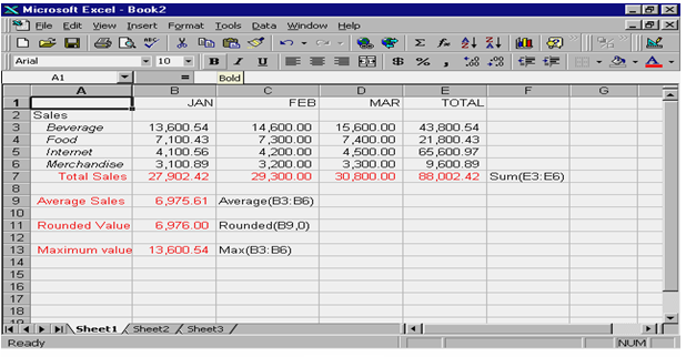
In the above example we have calculated the average of the values lying between B3 cell to B6, with the formula
=Average (B3:B6)
The SUM function
In the above example to calculate the sum of the values in the cells E3 to E6 the formula would be =SUM (E3:E6) or =E3+E4+E5+E6, the difference between the two is that in earlier on we have taken a range (a collection of consecutive cells) and calculated the sum by using the sum function and in the later we have simply added all the cells with the plus sign between them. Some Examples of the formulas are given in the figure.
The IF function
Returns one value if a condition we specify evaluates to TRUE and another value if it evaluates to FALSE. Use IF to conduct conditional tests on values and formulas.
IF (logical_test, value_if_true, value_if_false)
Logical_test is any value or expression that can be evaluated to TRUE or FALSE. For example, A10=100 is a logical expression; if the value in cell A10 is equal to 100, the expression evaluates to TRUE. Otherwise, the expression evaluates to FALSE. This argument can use any comparison calculation operator.
Value_if_true is the value that is returned if logical_test is TRUE. For example, if this argument is the text string “Within budget” and the logical_test argument evaluates to TRUE, then the IF function displays the text “Within budget”. If logical_test is TRUE and value_if_true is blank, this argument returns 0 (zero). To display the word TRUE, use the logical value TRUE for this argument. Value_if_true can be another formula.
Value_if_false is the value that is returned if logical_test is FALSE. For example, if this argument is the text string “Over budget” and the logical_test argument evaluates to FALSE, then the IF function displays the text “Over budget”. If logical_test is FALSE and value_if_false is omitted, (that is, after value_if_true, there is no comma), then the logical value FALSE is returned. If logical_test is FALSE and value_if_false is blank (that is, after value_if_true, there is a comma followed by the closing parenthesis), then the value 0 (zero) is returned. Value_if_false can be another formula.
Some points to be kept in mind while working with if function
- Up to seven IF functions can be nested as value_if_true and value_if_false arguments to construct more elaborate tests. See the following last example.
- When the value_if_true and value_if_false arguments are evaluated, IF returns the value returned by those statements.
- If any of the arguments to IF are arrays, every element of the array is evaluated when the IF statement is carried out.
Examples
On a budget sheet, cell A10 contains a formula to calculate the current budget. If the result of the formula in A10 is less than or equal to 100, then the following function displays “Within budget”. Otherwise, the function displays “Over budget”.
IF (A10<=100,”Within budget”,”Over budget”)
In the following example, if the value in cell A10 is 100, then logical_test is TRUE, and the total value for the range B5:B15 is calculated. Otherwise, logical_test is FALSE, and empty text (“”) is returned that blanks the cell that contains the IF function.
IF (A10=100,SUM (B5:B15),””)
Suppose an expense worksheet contains in B2:B4 the following data for “Actual Expenses” for January, February, and March: 1500, 500, 500. C2:C4 contains the following data for “Predicted Expenses” for the same periods: 900, 900, 925.
We can write a formula to check whether we are over budget for a particular month, generating text for a message with the following formulas
IF (B2>C2,”Over Budget”, ”OK”) equals “Over Budget”
IF (B3>C3,”Over Budget”, ”OK”) equals “OK”
Suppose we want to assign letter grades to numbers referenced by the name Average Score. See the following table. We can use the following nested IF function
| If Average Score is | Then return |
| Greater than 89 | A |
| From 80 to 89 | B |
| From 70 to 79 | C |
| From 60 to 69 | D |
| Less than 60 | F |
IF (Average Score>89,”A”, IF (Average Score>79,”B”,
IF (Average Score>69,”C”,
IF(Average Score>59,”D”,”F”))))
In the preceding example, the second IF statement is also the value_if_false argument to the first IF statement. Similarly, the third IF statement is the value_if_false argument to the second IF statement. For example, if the first logical_test (Average>89) is TRUE, “A” is returned. If the first logical_test is FALSE, the second IF statement is evaluated, and so on.
Worksheet functions using function wizard
Functions as discussed earlier can also be given with the help of function wizard also.
The VLOOKUP function
Searches for a value in the leftmost column of a table, and then returns a value in the same row from a column you specify in the table. Use VLOOKUP instead of HLOOKUP when your comparison values are located in a column to the left of the data you want to find. Its usage is
VLOOKUP (lookup_value, table_array, col_index_num, range_lookup)
Lookup_value is the value to be found in the first column of the array. Lookup_value can be a value, a reference, or a text string.
Table_array is the table of information in which data is looked up. Use a reference to a range or a range name, such as Database or List.
- If range_lookup is TRUE, the values in the first column of table_array must be placed in ascending order…, -2, -1, 0, 1, 2, …, A-Z, FALSE, TRUE; otherwise VLOOKUP may not give the correct value. If range_lookup is FALSE, table_array does not need to be sorted.
- You can put the values in ascending order by choosing the Sort command from the Data menu and selecting Ascending.
- The values in the first column of table_array can be text, numbers, or logical values.
- Uppercase and lowercase text is equivalent.
Col_index_num is the column number in table_array from which the matching value must be returned. A col_index_num of 1 returns the value in the first column in table_array; a col_index_num of 2 returns the value in the second column in table_array, and so on. If col_index_num is less than 1, VLOOKUP returns the #VALUE! error value; if col_index_num is greater than the number of columns in table_array, VLOOKUP returns the #REF! error value.
Range_lookup is a logical value that specifies whether you want VLOOKUP to find an exact match or an approximate match. If TRUE or omitted, an approximate match is returned. In other words, if an exact match is not found, the next largest value that is less than lookup_value is returned. If FALSE, VLOOKUP will find an exact match. If one is not found, the error value #N/A is returned.
If VLOOKUP can’t find lookup_value, and range_lookup is TRUE, it uses the largest value that is less than or equal to lookup_value. If lookup_value is smaller than the smallest value in the first column of table_array, VLOOKUP returns the #N/A error value. If VLOOKUP can’t find lookup_value, and range_lookup is FALSE, VLOOKUP returns the #N/A value.
More functions explained
| FUNCTIONS | Results |
| ABS | Returns the absolute value of a number |
| COUNTIF | Counts the number of non-blank cells with in a range |
| FACT | Returns the factorial of a number |
| MOD | Returns the remainder from division |
| POWER | Returns the result of a number raised to a power |
| PRODUCT | Multiplies the arguments |
| QUOTIENT | Returns the integer portion of a division |
| RAND | Returns a random number between 0 and 1 |
| ROUND | Rounds the number to a specified number of digits |
| SQRT | Returns a positive square root |
| SUM | Adds its arguments |
| SUMIF | Adds the cells specified by a given criteria |
| FREQUENCY | Returns a frequency distribution as a vertical array |
| MAX | Returns the maximum value in a list of arguments |
| MIN | Returns a minimum value in a list of arguments |
| MODE | Returns the most common value in a data set |
| PERCENTILE | Returns the Kth percentile of values in a range |
| VAR | Estimates variance based on a sample |
| FV | Returns the future value of an investment |
| IPMT | Returns the interest payment for an investment for a given period |
| PMT | Returns the periodic payment for an annuity |
| PPMT | Returns the payment on the principal for an investment for a given period |
| PV | Returns the present value of an investment |
| RATE | Returns the interest rate per period of an annuity |
| DATE | Returns the real number of a particular date |
| DAY | Converts a serial number to the day of the month |
| NOW | Returns the serial number of the current date and time |
| YEAR | Converts a serial number to a year |
| AND | Returns a true if all its arguments are true |
| IF | Specifies the logical test to perform |
| NOT | Reverses the logic if its arguments |
| OR | Returns true if any of the arguments is true |
| CONCATENATE | Joins the several text items into one text item |
| PROPER | Capitalizes the first letter in each word of a text value |
| REPLACE | Replaces characters within text |
| TRIM | Removes spaces from text |
| UPPER | Converts text to uppercase |
| VALUE | Converts a text argument to a number |
| HLOOKUP | Extract the database records row wise |
| VLOOKUP | Extracts the data base records column wise |
