Business Results for Projects

Business results are the outcomes which are measured and were identified during planning stage to show the impact of the project on organization. It involves performance measures for the business and the process involved.

Business Performance

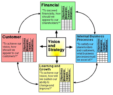
It is the crucial performance measure and balanced scorecard is used for it. Balanced scorecard was developed by Robert S. Kaplan and David P. Norton which focuses on four perspectives which are

1. Financial – It focuses relevant high-level financial measures and involves measuring cash flow, sales growth, operating income and return on equity.
2. Customer – It identifies measures which are customer facing like percent of sales from new products, on time delivery, share of important customers’ purchases, ranking by important customers.
3. Internal business processes – These measures answers the question “What must we excel at?” and include cycle time, unit cost, yield, new product introductions.
4. Learning and growth – It eyes continuity to improve, create value and innovate thus, involves measures like time to develop new generation of products, life cycle to product maturity, time to market versus competition.

Project Performance

It usually includes performance indexes on cost, schedule, defects per project, response time, etc. Two common measures are

1. Cost Performance Index – It is a measure of the efficiency of expenses spent on a project. It measures relationship between the budgeted cost of work performed (BCWP) and the actual work performed (ACWP) as a ratio.
2. Schedule Performance Index – SPI measures the success of project management to complete work on time. It is expressed as the ratio of the budgeted cost of work performed (BCWP) to the budgeted cost of work scheduled (BCWS).

Process Performance

It is a measure of an organization’s activities and performance and includes metrics as

1. Percentage Defective – This is defined as the (Total number of defective parts)/(Total number of parts) X 100. So if there are 1,000 parts and 10 of those are defective, the percentage of defective parts is (10/1000) X 100 = 1%
2. PPM – It is same as the ratio defined in percentage defective, but multiplied by 1,000,000 and PPM for above example is 10,000. It indicates of presence of one or more defects only.
3. Defects per Unit (DPU) – It finds the average number of defects per unit which also needs categorization of the units into number of defects from 0, 1, 2, up to the maximum number. As an example, the below chart shows defect count for 100 units with maximum of 5 defects.

Defects	0	1	2	3	4	5
# of Units	70	20	5	4	9	1

The average number of defects is DPU = [Sum of all (D * U)]/100 =

[(0 * 70) + (1 * 20) + (2 * 5) + (3 * 4) + (4 * 9) + (5 * 1)]/100 = 47/100 = 0.47

1. Defects per Opportunity (DPO) – It focus on number of ways of a defect occurrence or the defect “opportunity”, similar to a failure mode in FMEA. As an example from previous data considering that each unit can have a defect occurrence in one of 6 possible ways. Then the number of opportunities for a defect in each unit is 6 and DPO = DPU/O = 0.47/6 = 0.078333
2. Defects per Million Opportunities (DPMO) – It is obtained by multiplying DPO by 1,000,000 as DPMO = DPO * 1,000,000 = 0.078333 * 1,000,000 = 78,333
3. Rolled Through Yield (RTY) – A yield measures the probability of a unit passing a step defect-free, and the rolled throughput yield (RTY) measures the probability of a unit passing a set of processes defect-free. This takes the percentage of units that pass through several sub-processes of an entire process without a defect. The number of units without a defect is equal to the number of units that enter a process minus the number of defective units. For illustration, the number of units given as an input to a process is P, the number of defective units is D then, the first-pass yield for each sub-process or FPY is equal to (P – D)/P. After getting FPY for each sub-process, multiply them altogether to obtain RTY as, the yields of 4 sub-processes are 0.994, 0.987, 0.951 and 0.990, then the RTY = (0.994)(0.987)(0.951)(0.990) = 0.924 or 92.4%.
4. Sigma Level- A Six Sigma process is the output of process that has a mean of 0 and standard deviation of 1, with an upper specification limit (USL) and lower specification limit (LSL) set at +3 and -3. However, there is also the matter of the 1.5-sigma shift which occurs over the long term. After computing DPMO and RTY, the sigma level can also be computed as

If yield is	DPMO is	Sigma Level is
30.9%	690,000	1.0
62.9%	308,000	2.0
93.3	66,800	3.0
99.4	6,210	4.0
99.98	320	5.0
99.9997	3.4	6.0

1. Cost of poor quality – It is also called as the cost of nonconformance, which includes the cost of all defects as
2. Internal defects – Before product leaves the organization and includes scrapping, repairing, or reworking the parts.
3. External defects – After product leaves the organization and includes costs of warranty, returned merchandise, or product liability claims and lawsuits.

It is difficult to calculate because the external costs can be delayed by months or even years after the products are sold thus, the internal costs of poor quality are computed.

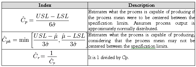
1. Process Capability – It compares the output of an in-control process to the specification limits by using capability indices. The comparison is made by forming the ratio of the spread between the process specifications (the specification “width”) to the spread of the process values, as measured by 6 process standard deviation units (the process “width”). It is used to compare the output of a stable process with the process specifications and make a statement about how well the process meets specification. There are several statistical measures that are used to measure the capability of a process as Cp, Cpk and Cr.

FMEA and RPN

Failure Mode and Effects Analysis (FMEA) is computed for failure analysis which also involves Risk Priority Number (RPN) computation. Both have been explained earlier.

Six Sigma Metrics

There are many metrics used in Six and they can operate in different ways. For example, defects per unit (DPU), which involves such considerations as how well your company is performing within your specification limits for your customer and how many defects per million opportunities do your processes actually generate. There’s also first time yield, which could include the number of calls your company can handle on the first attempt at a contact center or the percentage of good quality products produced during your manufacturing process.

Rolled through yield (RTY) is a metric that examines the quality of the finished item. In an automotive assembly plant, for example, you would examine the percentage of good quality production at each station in the assembly. Cycle time also covers important areas, such as the order delivery time from a customer order to actual delivery, the delivery time from cash to cash, the time taken to perform a task, and how much variation is found. Finally, cost of poor quality (COPQ) concerns issues such as the cost of scrap, where you work, returns, making goods, and delivery expediting.

Counting defects is an important task and there are many ways to use the various data that is gathered during the Six Sigma process. You want to examine the outputs of your process very carefully, so it’s here that you must pay a lot of attention to capturing discrete data. Examples of discrete data may include

1. elapsed time to provide a service or to do a task
2. the weight, color, or dimension of an item
3. the amount of scrap resulting at a given step in a process
4. the percentage of rework required for each task
5. the number of complaints received from your customers about delivering a particular product or service

DPU

It’s important have a good understanding of the number of defects statistically found per unit and what the average number of defects are that you find in your sample. For example, with a really simple part with a single dimension cut in the CNC machine, you might find that you have a tiny fraction of a number, such as .00 something defects per unit.

However, if you had 50 different things you were cutting in the part or were delivering a complex machine, such as building an entire piece of equipment, and considered all the defects that could be found in that process, you could find that the defects per unit is above 5, 10, or even 100 types of defects per unit over time.

The reason for calculating DPU is to get a baseline and common benchmark. You need to know where you are, how that compares, and what the customer expects. DPU gives you an understanding of the current situation and which processes were evaluated. From there, you need to identify your future improvement activities. This could be done using several tools:

1. the customer voice – what the customer actually cares about
2. cost data about what the impacts are in terms of your cost
3. Pareto analysis – to zero in on the vital few areas where you get the biggest bang for your buck with your improvement activities; also to identify non-conformance and areas where you need to improve your controls so that you can get repeatable results out of this process

An example of defects per unit can be seen with caps on bottles that won’t seal. This is the function of the number of defects you actually find divided by the number of units that you inspect. Before performing that calculation, it’s important to know exactly what constitutes a defect and identify a clear unit of measure for your specific situation. In this case, the defect is a cap that won’t seal and the unit is a bottle.

If you had a confidence interval and wanted to get at least 50% with a population of one million bottles; if you want to be 95% confident with a confidence interval of 0.1, you need to take at least 97 samples. If you inspect them and find out that you had zero defects, then you would be pretty confident that it would be at least 95% good most of the time. If you want to get to 99% confident, you would need to inspect at least 166 samples to have the confidence factor of knowing statistically how well you are performing with respect to the defects per unit calculation.

Parts per million (PPM)

Parts per million also plays an important role in finding defects:

1. First, you do a basic calculation of the number of defects observed versus the number of units inspected.
2. Then, you multiply that by one million to get to the PPM.

For example, a manager of a fast food restaurant might observe that there are 15 defective results with 100 customers that pass through and what that manager can now do is simply calculate the PPM by taking the product of 115 divided by 100 times one million. That gives him a PPM of 150,000. By multiplying this factor of 15 divided by 100 by one million, he can then extrapolate this and decide if he is happy with 150,000 of every million customers a year having a poor experience of the company’s quality. So, he has to think about how many customers are impacted and if that’s an acceptable number, or whether he needs to target improvement.

DPMO

Defects per million opportunities, or DPMO, measures the mathematical possibility that a process can be defective. This allows you to standardize on defects at the opportunity level and it enables the comparison of complex processes from one to the other. For example, you might use defects per million opportunities for each step in a complex product or process to examine the aggregated risk of a defect or a defective at the end of the process. This is not unlike the notion of a rolled throughput yield of a process. You could add up the defect parts per million opportunities across the process and then compare process A to process B to get a sense of what really needs attention first, especially if the values between the two are dramatically different.

There are three major components to DPMO and to understand this, you have to recognize that the DPMO calculation looks at opportunities for defects within the units that result in products or services that fail to meet the customer’s requirements and performance standards. There are three key pieces that make up the DPMO calculation:

1. the measurable failure or the defect being found
2. the unit, final deliverable, product, or service impacted by the nature of defects that you find
3. the opportunity for that measurable attribute within the unit that could result in a defect

The formula for defects per million opportunities (DPMO) is the number of defects found in a sample, divided by the total number of defect opportunities found in the sample, multiplied by one million. To illustrate this, consider a sample of 1,000 units, in which there are 50 defects. You divide 50 defects by 1,000 units and get a factor of 0.05. You then multiply 0.05 by one million opportunities, which results in a DPMO of 50,000.

Sigma Level 

To better understand the sigma level, you need to know the DPMO numbers and the corresponding sigma values. A DPMO of 690,000 equates to 1.0 sigma; a DPMO of 308,000 is 2.0 sigma; 66,800 is 3.0 sigma; 6,210 is 4.0 sigma; 320 is 5.0 sigma; and 3.4 is 6.0 sigma. In the example with the DPMO calculation of 15,000, the sigma level falls between 3 and 4. On a bell-shaped curve, that’s plus or minus three standard deviations to the left and to the right of the mean.

FTY

Yield is basically the percentage of error-free output at a given step of a process or the output that is good the first time. It looks at a production or service with more than a single step, where there can be defects as well.

Yield is calculated in two different ways: first time yield (FTY) and rolled throughput yield (RTY). FTY is looked at for an individual step in a process, whereas the RTY could look at the entire end-to-end process.

For example, in an automotive assembly plant, at each of the stations measured, you would find out what percentage of the time you fail in moving through a process. Through examining these results, you might find that the FTY for the entire automotive assembly plant was only about 21%, meaning 79% of everything going through the stations needed to be reworked or fixed before it got to the end of the line. This would give you a basis to go back and look at which few stations within the entire plan really needed the most attention, so that you can improve the overall RTY.

First time yield (FTY)

With FTY, consider how you would calculate it on a first pass yield. If you have 10,000 units entering a step in the process and you find out that you lose, scrap, or rework 1,000 units as you go through the process, you end up with 9,000 units at the backend. If you do the calculation of the 9,000 divided by the time, you find out that your FTY, would be 90%.

RTY

Rolled throughput yield (RTY) is more useful as a management metric than just first time yield (FTY). For example, a process has 1,000 units and 100 are scrapped at Step 1. This calculates as .9 or 90% first time through. There are 50 units scrapped at Step 2, which results in 94% first time through. When the process reaches Step 10, 795 units enter the process and 690 units exit as a good product at the end, with 87% first time through.

RTY formula

The formula for rolled throughput yield is a function of multiple FTY calculations, each successively multiplied by the other through a series. For example, RTY is equal to FTY sub 1, multiplied by FTY sub 2, multiplied by FTY sub 3, multiplied by FTY sub 4, and so on.

Looking at sample data, your process is running at .987 or 98.7% first time through for a given step in the process times two successive steps. When decimals are multiplied, the result is reduced – .987 multiplied by .958 multiplied by .996 is equal to .942 multiplied by 100. This results in a RTY percentage of 94.2%. Each step in this three-step process has an FTY well above 90%. Judging from these percentages, it seems the overall process is doing well. However, by rolling the yield through from one step to another in the process, a different picture is revealed. A calculation shows that the RTY is only about 84.9%. Approximately 15% of everything going through this process is being scrapped. The first time pass of 95 multiplied by 92.6 equals 88, and multiply 88 by 96.6 and that returns a result of 85. This is the cumulative RTY calculation.

COPQ

Costs occur due to low quality products, activities that do not meet desired outcomes, and inefficiency-related costs. Understanding the true cost of poor quality (COPQ) of a company is something even the very best companies struggle to get a handle on.

These costs are all the combined visible and hidden costs that eat into the profit margins of the organization:

1. having activities that don’t meet the desired outcomes and increase inefficiency
2. slowing down dramatically to get good quality versus the rate you should be running at
3. spending a lot of resources on rework instead of making things right the first time

COPQ is the actual cost minus the minimum cost. You can use statistics understand this measure of quality from many different perspectives. It’s really important to understand that for a non-Six Sigma kind of process, the cost can be extremely high for quality. A company running at 4 sigma can see as much as 20% of sales revenues going to waste, and at 5 sigma, a company could lose 10% of sales revenue. Some of the largest companies in the world could easily be operating at $8 billion to $12 billion in losses per year all around this cost of poor quality.

You need to look at what your current sigma level is, understand your true current cost of quality at the Define stage, and get a really clear project charter about what you are trying to accomplish. You then have the basis to track the benefits post project and use that to prioritize the portfolio of projects for the things to be done first, second, third, and fourth.

The other thing you get out of this is a really useful analysis tool. If you look at yield, you look at defects – defective parts per million and the sigma that you are operating at. For example, a 3.1 sigma would probably run at an exposure of 30% for the cost of poor quality for an organization. As you improve to 3.5 sigma, still as much as 20% is wasted. At 4.6 sigma, there’s a waste of 10%, and 4.98 sigma has a waste of 5%. As you improve your sigma performance and drive down the cost of quality, you should also consider what that does for you in other ways. For example, what it’s doing to customer satisfaction, and what it’s doing for market share and top line growth. As you move from 30% to 10% or less cost of poor quality, you are going to see a lot of benefit for the entire organization.

Cycle Time

Understanding and managing cycle time and lead time is important for organizations that need time to respond to their customers. These have a major effect on productivity which stimulates competitiveness in the marketplace. It’s also important to understand the difference between lead time for an overall process versus cycle time of the various steps.

In one example, when posting an article online, the cycle time for a task – meet with author – is a two days. However, this task is only part of a bigger picture of understanding the end-to-end process cycle time of 14 days, which is made up of several activities across the value string. Each activity has its own cycle time. The tasks in this example process are – meet with author, read/approve manuscript, proof stage(s), do final proofread, and post to Internet. Each has their own cycle time. If you did the value stream map, you would have these high-level headers for the activities going on. It takes two days to meet with authors, three days to move through and look at manuscripts, five days to move through the proofing stage, and then 2 days doing final proofreading and 2 days to be ready to post the article or blog to the Internet. This relates to all the material you are going to push out to the marketplace to market the products and services that you offer.

An example process for the manufacture of precision tools has three steps: attach lever, inspect, and pack. Sample columns in a worksheet show six observed times for each step. Further key parts of data can be included as well, such as the most frequently recurring value. In this example, for the attach lever task, the observed time of 3 seconds was present in three different columns. For the inspect task, the observed time of 2 seconds was present in three different columns. Further data, such as the highest value observed in each task, can also be recorded in addition to the low repeat time.

There are benefits to understanding each type of data. The most frequent value is probably the one that can be repeated without difficulty by operators, the high time helps you understand the worst case scenario regarding the amount of variation possible, and the low repeat reflects the best case scenario. If you are under pressure to actually improve performance, then you may want to use lean Six Sigma tools to perform repeatedly at this level.

You could have multiple operators performing the same work simultaneously or a single operator performing multiple tasks. Your cycle time worksheet needs to be designed to reflect the actual production processes in your organization. The aim is to establish the most frequently recurring time.

Takt Time

Takt time is the required rate of production. It is usually expressed as a function of how many units per hour are needed but it could be also be expressed over days, weeks, or even months. Process cycle time needs to be balanced to meet the takt time so that you’re not overtasking or underutilizing your resources. If your cycle time is greater than your takt time, you’re going to have a problem.

For example, if the takt time is 10 minutes but the cycle time is actually 15 minutes, you won’t meet customer demand. You can use lean Six Sigma tools to break that bottleneck or figure out how to do work balancing and divide that work differently. Conversely, if the cycle time is less than takt time, you run the risk of having idle resources waiting for work to do while trying to operate at the production pace the customer requires.

Consider an example calculation of a process that produces goods. You need to remember to include the time that operators spend on breaks, meetings and other activities, since customers would be placing work orders regardless of whether the operators are on break or not. In this example, the customer demand rate is 120 units per day and you work an 8-hour shift which is 480 minutes. When 480 minutes is divided by 120, the result is a takt time of 4 minutes per unit that you need to produce at to maintain the rate that customers are demanding. Usually shift length would only be used once the time spent on breaks and lunches are subtracted. So if you are going to lose 40 minutes a day for breaks, you would change the calculation to divide by 440 instead of 480. That would give you a different result with 4.5 minutes average takt time. This is the time that you want to look at, so that you are actually running and paying attention to the day-to-day and hour-to-hour production. This time is a better number to use to know whether you are keeping up with the work.