A large number of problems in production planning and scheduling, location, transportation, finance, and engineering design require that decisions be made in the presence of uncertainty. Uncertainty, for instance, governs the prices of fuels, the availability of electricity, and the demand for chemicals. A key difficulty in optimization under uncertainty is in dealing with an uncertainty space that is huge and frequently leads to very large-scale optimization models. Decision-making under uncertainty is often further complicated by the presence of integer decision variables to model logical and other discrete decisions in a multi-period or multi-stage setting.
Approaches to optimization under uncertainty have followed a variety of modeling philosophies, including expectation minimization, minimization of deviations from goals, minimization of maximum costs, and optimization over soft constraints. The main approaches to optimization under uncertainty are: stochastic programming (recourse models, robust stochastic programming, and probabilistic models), fuzzy programming (flexible and possibilistic programming), and stochastic dynamic programming. Then, we review applications and the state-of-the-art in computations, as well as important algorithmic developments by the process systems engineering community.
It is a framework for modeling optimization problems that involve uncertainty. Whereas deterministic optimization problems are formulated with known parameters, real world problems almost invariably include some unknown parameters. When the parameters are known only within certain bounds, one approach to tackling such problems is called robust optimization. Here the goal is to find a solution which is feasible for all such data and optimal in some sense. Stochastic programming models are similar in style but take advantage of the fact that probability distributions governing the data are known or can be estimated. The goal here is to find some policy that is feasible for all (or almost all) the possible data instances and maximizes the expectation of some function of the decisions and the random variables. More generally, such models are formulated, solved analytically or numerically, and analyzed in order to provide useful information to a decision-maker.
As an example, consider two-stage linear programs. Here the decision maker takes some action in the first stage, after which a random event occurs affecting the outcome of the first-stage decision. A recourse decision can then be made in the second stage that compensates for any bad effects that might have been experienced as a result of the first-stage decision. The optimal policy from such a model is a single first-stage policy and a collection of recourse decisions (a decision rule) defining which second-stage action should be taken in response to each random outcome.
Stochastic programming has applications in a broad range of areas ranging from finance to transportation to energy optimization.
Two-Stage Problems
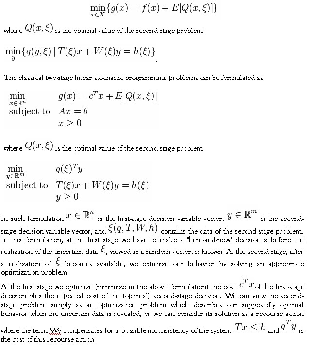
Under the standard two-stage stochastic programming paradigm, the decision variables of an optimization problem under uncertainty are partitioned into two sets. The first-stage variables are those that have to be decided before the actual realization of the uncertain parameters. Subsequently, once the random events have presented themselves, further design or operational policy improvements can be made by selecting, at a certain cost, the values of the second-stage, or recourse , variables. Traditionally, the second-stage variables are interpreted as corrective measures or recourse against any infeasibilities arising due to a particular realization of uncertainty. However, the second-stage problem may also be an operational-level decision problem following a first-stage plan and the uncertainty realization. Due to uncertainty, the second-stage cost is a random variable. The objective is to choose the first-stage variables in a way that the sum of the first-stage costs and the expected value of the random second-stage costs is minimized. The concept of recourse has been applied to linear, integer, and non-linear programming.
The basic idea of two-stage stochastic programming is that (optimal) decisions should be based on data available at the time the decisions are made and should not depend on future observations. Two-stage formulation is widely used in stochastic programming. The general formulation of a two-stage stochastic programming problem is given by:
The considered two-stage problem is linear because the objective functions and the constraints are linear. Conceptually this is not essential and one can consider more general two-stage stochastic programs. For example, if the first-stage problem is integer, one could add integrality constraints to the first-stage problem so that the feasible set is discrete. Non-linear objectives and constraints could also be incorporated if needed.
Recourse Models
When some of the data is random, then solutions and the optimal objective value to the optimization problem are themselves random. A distribution of optimal decisions is generally unimplementanble (what do you tell your boss?). Ideally, we would like one decision and one optimal objective value.
One logical way to pose the problem is to require that we make one decision now and minimize the expected costs (or utilities) of the consequences of that decision. This paradigm is called the recourse model. Suppose x is a vector of decisions that we must take, and y(w) is a vector of decisions that represent new actions or consequences of x. Note that a different set of y’s will be chosen for each possible outcome w. The Two-Stage formulation is
minimize f1(x) + Expected Value[ f2( y(w), w ) ]
subject to g1(x) <= 0, … gm(x) <= 0
h1(x, y(w) ) <= 0 for all w in W
..
hk(x, y(w) ) <= 0 for all w in W
x in X, y(w) in Y
The set of constraints h1 … hk describe the links between the first stage decisions x and the second stage decisions y(w). Note that we require that each constraint hold with probability 1, or for each possible w in W. The functions f2 are quite frequently themselves the solutions of mathematical problems. We don’t want to make an arbirary correction (recourse) to the first stage decision; we want to make the best such correction.
Recourse models can be extended in a number of ways. One of the most common is to include more stages. With a multistage problem, we in effect make one decision now, wait for some uncertainty to be resolved (realized), and then make another decision based on what’s happened. The objective is to minimize the expected costs of all decisions taken.
Solving Recourse Problems – Solving a recourse problem is generally much more difficult than the determinsitic version. The hardest part is to evaluate the expected costs of each stage (except the first). In effect, we’re trying to perform high-dimensional numerical integration on the solutions to mathematical programs.
When the random data is discretely distributed, the problem can be written as a large deterministic problem. The expectations can be written as finite sums, and each constraint can be duplicated for each realization of the random data. The resulting deterministic equivalent problem can be solved using any general purpose optimization package.
When the random data has a continuous distribution, the integrals are particularly difficult. However, you can find upper and lower bounds to the expected recourse cost that reduce to discretely distributed stochastic programs.
