Drawing statistical conclusions involves usage of enumerative and analytical studies, which are
Enumerative or descriptive studies describes data using math and graphs and focus on the current situation like a tailor taking a measurement of length, is obtaining quantifiable information which is an enumerative approach. Enumerative data is data that can be counted. These studies are used to explain data, usually sample data in central tendency (median, mean and mode), variation (range and variance) and graphs of data (histograms, box plots and dot plots). Measures calculate from a sample, called statistics with which these measures describe a population, called as parameters.
A statistic is a quantity derived from a sample of data for forming an opinion of a specified parameter about the target population. A sample is used as data on every member of population is impossible or too costly. A population is an entire group of objects that contains characteristic of interest. A population parameter is a constant or coefficient that describes some characteristic of a target population like mean or variance.
Analytical (Inferential) Studies – The objective of statistical inference is to draw conclusions about population characteristics based on the information contained in a sample. It uses sample data to predict or estimate what a population will do in the future like a doctor taking a measurement like blood pressure or heart beat to obtain a causal explanation for some observed phenomenon which is an analytic approach.
It entails define the problem objective precisely, deciding if it will be evaluated by a one or two tail test, formulating a null and an alternate hypothesis, selecting a test distribution and critical value of the test statistic reflecting the degree of uncertainty that can be tolerated (the alpha, beta, risk), calculating a test statistic value from the sample and comparing the calculated value to the critical value and determine if the null hypothesis is to be accepted or rejected. If the null is rejected, the alternate must be accepted. Thus, it involves testing hypotheses to determine the differences in population means, medians or variances between two or more groups of data and a standard and calculating confidence intervals or prediction intervals.
Various statistics terminologies which are used extensively are
- Data – facts, observations, and information that come from investigations.
- Measurement data sometimes called quantitative data — the result of using some instrument to measure something (e.g., test score, weight);
- Categorical data also referred to as frequency or qualitative data. Things are grouped according to some common property(ies) and the number of members of the group are recorded (e.g., males/females, vehicle type).
- Variable – property of an object or event that can take on different values. For example, college major is a variable that takes on values like mathematics, computer science, etc.
- Discrete Variable – a variable with a limited number of values (e.g., gender (male/female).
- Continuous Variable – It is a variable that can take on many different values, in theory, any value between the lowest and highest points on the measurement scale.
- Independent Variable – a variable that is manipulated, measured, or selected by the user as an antecedent condition to an observed behavior. In a hypothesized cause-and-effect relationship, the independent variable is the cause and the dependent variable is the effect.
- Dependent Variable – a variable that is not under the user’s control. It is the variable that is observed and measured in response to the independent variable.
Central limit theorem and sampling distribution of the mean
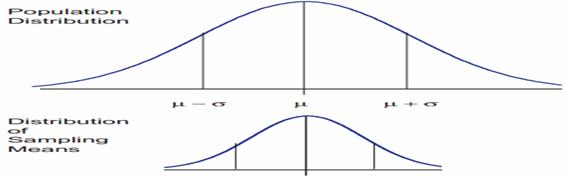
The central limit theorem is the basis of many statistical procedures. The theorem states that for sufficiently large sample sizes ( n ≥ 30), regardless of the shape of the population distribution, if samples of size n are randomly drawn from a population that has a mean µ and a standard deviation σ , the samples’ means X are approximately normally distributed. If the populations are normally distributed, the sample’s means are normally distributed regardless of the sample sizes. Hence, for sufficiently large populations, the normal distribution can be used to analyze samples drawn from populations that are not normally distributed, or whose distribution characteristics are unknown. The theorem states that this distribution of sample means will have the same mean as the original distribution, the variability will be smaller than the original distribution, and it will tend to be normally distributed.
When means are used as estimators to make inferences about a population’s parameters and n ≥ 30, the estimator will be approximately normally distributed in repeated sampling. The mean and standard deviation of that sampling distribution are given as µx = µ and σx = σ/√n. The theorem is applicable for controlled or predictable processes. Most points on the chart tend to be near the average with the curve’s shape is like bell-shaped and the sides tend to be symmetrical. Using ± 3 sigma control limits, the central limit theorem is the basis of the prediction as, if the process has not changed, a sample mean falls outside the control limits an average of only 0.27% of the time. The theorem enables the use of smaller sample averages to evaluate any process because distributions of sample means tend to form a normal distribution.
Measurement
A measurement is assigning numerical value to something, usually continuous elements. Measurement is a mapping from an empirical system to a selected numerical system. The numerical system is manipulated and the results of the manipulation are studied to help the manager better understand the empirical system. Measured data is regarded as being better than counted data. It is more precise and contains more information. Sometimes, data will only occur as counted data. If the information can be obtained as either attribute or variables data, it is generally preferable to collect variables data.
The information content of a number is dependent on the scale of measurement used which also determines the types of statistical analyses. Hence, validity of analysis is also dependent upon the scale of measurement. The four measurement scales employed are nominal, ordinal, interval, and ratio and are summarized as
| Scale | Definition | Example | Statistics |
| Nominal | Only the presence/absence of an attribute. It can only count items. Data consists of names or categories only. No ordering scheme is possible. It has central location at mode and only information for dispersion. | go/no-go, success/fail, accept/reject | percent, proportion, chi-square tests |
| Ordinal | Data is arranged in some order but differences between values cannot be determined or are meaningless. It can say that one item has more or less of an attribute than another item. It can order a set of items. It has central location at median and percentages for dispersion. | taste, attractiveness | rank-order correlation, sign or run test |
| Interval | Data is arranged in order and differences can be found. However, there is no inherent starting point and ratios are meaningless. The difference between any two successive points is equal; often treated as a ratio scale even if assumption of equal intervals is incorrect. It can add, subtract and order objects. It has central location at arithmetic mean and standard deviation for dispersion. | calendar time, temperature | correlations, t-tests, F-tests, multiple regression |
| Ratio | An extension of the interval level that includes an inherent zero starting point. Both differences and ratios are meaningful. True zero point indicates absence of an attribute. It can add, subtract, multiply and divide. It has central location at geometric mean and percent variation for dispersion. | elapsed time, distance, weight | t-test, F-test, correlations, multiple regression |
