It is the least squares estimator of a linear regression model with a single explanatory variable. In other words, simple linear regression fits a straight line through the set of n points in such a way that makes the sum of squared residuals of the model (that is, vertical distances between the points of the data set and the fitted line) as small as 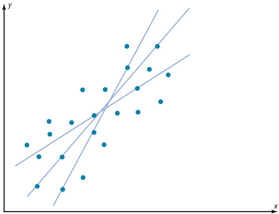
Given a scatter plot, you must be able to draw the line of best fit. Best fit means that the sum of the squares of the vertical distances from each point to the line is at a minimum.
Basic Equation for Regression – Observed Value = Fitted Value + Residual
The least squares line is the line that minimizes the sum of the squared residuals. It is the line quoted in regression outputs.
The reason you need a line of best fit is that the values of y will be predicted from the values of x; hence, the closer the points are to the line, the better the fit and the prediction will be. When r is positive, the line slopes upward and to the right. When r is negative, the line slopes downward from left to right.
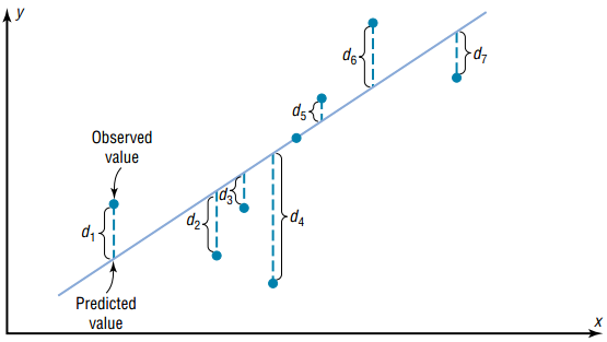
A fitted value is the predicted value of the dependent variable. Graphically, it is the height of the line above a given explanatory value. The corresponding residual is the difference between the actual and fitted values of the dependent variable.
In algebra, the equation of a line is usually given as y = mx+ b, where m is the slope of the line and b is the y intercept. In statistics, the equation of the regression line is written as y’ = a + bx , where a is the y’ intercept and b is the slope of the line.
There are several methods for finding the equation of the regression line. These formulas use the same values that are used in computing the value of the correlation coefficient.
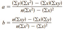
Formulas for the Regression Line y’ = a + bx
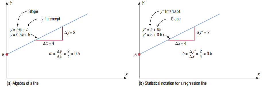
where a is the y’ intercept and b is the slope of the line.
Residual Analysis and Regression Assumptions
Regression Assumptions
Classical assumptions for regression analysis include:
- The sample is representative of the population for the inference prediction.
- The error is a random variable with a mean of zero conditional on the explanatory variables.
- The independent variables are measured with no error. (Note: If this is not so, modeling may be done instead using errors-in-variables model techniques).
- The independent variables (predictors) are linearly independent, i.e. it is not possible to express any predictor as a linear combination of the others.
- The errors are uncorrelated, that is, the variance–covariance matrix of the errors is diagonal and each non-zero element is the variance of the error.
- The variance of the error is constant across observations (homoscedasticity). If not, weighted least squares or other methods might instead be used.
These are sufficient conditions for the least-squares estimator to possess desirable properties; in particular, these assumptions imply that the parameter estimates will be unbiased, consistent, and efficient in the class of linear unbiased estimators.
Residual Analysis
Residual (or error) represents unexplained (or residual) variation after fitting a regression model. It is the difference (or left over) between the observed value of the variable and the value suggested by the regression model.
The difference between the observed value of the dependent variable (y) and the predicted value (ŷ) is called the residual (e). Each data point has one residual.
Residual = Observed value – Predicted value
e = y – ŷ
Both the sum and the mean of the residuals are equal to zero. That is, Σ e = 0 and e = 0.
Analyse residuals from regression – An important way of checking whether a regression, simple or multiple, has achieved its goal to explain as much variation as possible in a dependent variable while respecting the underlying assumption, is to check the residuals of a regression. In other words, having a detailed look at what is left over after explaining the variation in the dependent variable using independent variable(s), i.e. the unexplained variation.
Most problems that were initially overlooked when diagnosing the variables in the model or were impossible to see, will, turn up in the residuals, for instance:
- Outliers that have been overlooked, will show up … as, often, very big residuals.
- If the relationship is not linear, some structure will appear in the residuals
- Non-constant variation of the residuals (heteroscedasticity)
- If groups of observations were overlooked, they’ll show up in the residuals
In one word, the analysis of residuals is a powerful diagnostic tool, as it will help you to assess, whether some of the underlying assumptions of regression have been violated.
Tools for analyzing residuals – For the basic analysis of residuals you will use the usual descriptive tools and scatterplots (plotting both fitted values and residuals, as well as the dependent and independent variables you have included in your model.
- A histogram, dot-plot or stem-and-leaf plot lets you examine residuals
- A Q-Q Plot to assess normality of the residuals.
- Plot the residuals against the dependent variable to zoom on the distances from the regression line.
- Plot the residuals against each independent variables to find out, whether a pattern is clearly related to one of the independents.
- Plot the residuals against other variables to find out, whether a structure appearing in the residuals might be explained by another variable (a variable that you might want to include into a more complex model.
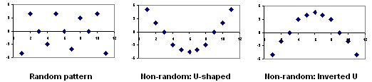
Residual Plots – A residual plot is a graph that shows the residuals on the vertical axis and the independent variable on the horizontal axis. If the points in a residual plot are randomly dispersed around the horizontal axis, a linear regression model is appropriate for the data; otherwise, a non-linear model is more appropriate.
Below the table on the left shows inputs and outputs from a simple linear regression analysis, and the chart on the right displays the residual (e) and independent variable (X) as a residual plot.
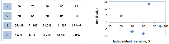
The residual plot shows a fairly random pattern – the first residual is positive, the next two are negative, the fourth is positive, and the last residual is negative. This random pattern indicates that a linear model provides a decent fit to the data.
Below, the residual plots show three typical patterns. The first plot shows a random pattern, indicating a good fit for a linear model. The other plot patterns are non-random (U-shaped and inverted U), suggesting a better fit for a non-linear model.