A population is identified with the goal of estimating the (unknown) population mean value, identified by µ. You select a random or representative sample from the population where, for notational convenience, the sample measurements are identified as Y1, Y2, …, Yn, where n is the sample size.
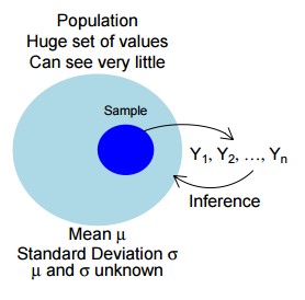
Given the data, the best estimate, of µ is the sample mean
There are two main methods for inferences on µ: confidence intervals (CI) and hypothesis tests. The standard CI and test procedures are based on Y and s, the sample standard deviation.
Two-sample hypothesis testing is statistical analysis designed to test if there is a difference between two means from two different populations. For example, a two-sample hypothesis could be used to test if there is a difference in the mean salary between male and female doctors in the New York City area.
A two-sample hypothesis test could also be used to test if the mean number of defective parts produced using assembly line A is greater than the mean number of defective parts produced using assembly line B. Similar to one-sample hypothesis tests, a one-tailed or two-tailed test of the null hypothesis can be performed in two-sample hypothesis testing as well. The two-sample hypothesis test of no difference between the mean salaries of male and female doctors in the New York City area is an example of a two-tailed test. The test of whether or not the mean number of defective parts produced on assembly line A is greater than the mean number of defective parts produced on assembly line B is an example of a one-tailed test.
Analysis of variance (ANOVA) is a collection of statistical models used to analyze the differences among group means and their associated procedures (such as “variation” among and between groups). The observed variance in a particular variable is partitioned into components attributable to different sources of variation. In its simplest form, ANOVA provides a statistical test of whether or not the means of several groups are equal, and therefore generalizes the t-test to more than two groups. As doing multiple two-sample t-tests would result in an increased chance of committing a statistical type I error, ANOVAs are useful for comparing (testing) three or more means (groups or variables) for statistical significance.
ANOVA is a particular form of statistical hypothesis testing heavily used in the analysis of experimental data. A test result (calculated from the null hypothesis and the sample) is called statistically significant if it is deemed unlikely to have occurred by chance, assuming the truth of the null hypothesis. A statistically significant result, when a probability (p-value) is less than a threshold (significance level), justifies the rejection of the null hypothesis, but only if the a priori probability of the null hypothesis is not high.
In the typical application of ANOVA, the null hypothesis is that all groups are simply random samples of the same population. For example, when studying the effect of different treatments on similar samples of patients, the null hypothesis would be that all treatments have the same effect (perhaps none). Rejecting the null hypothesis would imply that different treatments result in altered effects.
By construction, hypothesis testing limits the rate of Type I errors (false positives) to a significance level. Experimenters also wish to limit Type II errors (false negatives). The rate of Type II errors depends largely on too small of sample size, significance level (when the standard of proof is high, the chances of overlooking a discovery are also high) and effect size.
The reason for doing an ANOVA is to see if there is any difference between groups on some variable. For example, you might have data on student performance in non-assessed tutorial exercises as well as their final grading. You are interested in seeing if tutorial performance is related to final grade. ANOVA allows you to break up the group according to the grade and then see if performance is different across these grades. ANOVA is available for both parametric (score data) and non-parametric (ranking/ordering) data.
Types of ANOVA
One-way between groups – The example given above is called a one-way between groups model. You are looking at the differences between the groups. There is only one grouping (final grade) which you are using to define the groups. This is the simplest version of ANOVA. This type of ANOVA can also be used to compare variables between different groups – tutorial performance from different intakes.
One-way repeated measures – A one-way repeated measures ANOVA is used when you have a single group on which you have measured something a few times. For example, you may have a test of understanding of Classes. You give this test at the beginning of the topic, at the end of the topic and then at the end of the subject. You would use a one-way repeated measures ANOVA to see if student performance on the test changed over time.
Two-way between groups – A two-way between groups ANOVA is used to look at complex groupings. For example, the grades by tutorial analysis could be extended to see if overseas students performed differently to local students. What you would have from this form of ANOVA is
- The effect of final grade
- The effect of overseas versus local
- The interaction between final grade and overseas/local
Each of the main effects are one-way tests. The interaction effect is simply asking “is there any significant difference in performance when you take final grade and overseas/local acting together”.
Two-way repeated measures – This version of ANOVA simple uses the repeated measures structure and includes an interaction effect. In the example given for one-way between groups, you could add Gender and see if there was any joint effect of gender and time of testing – i.e. do males and females differ in the amount they remember/absorb over time.
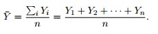
In the illustrations, each group is identified as X1, X2, etc. In the first illustration, we divide the dogs according to the product (interaction) of two binary groupings: young vs old, and short-haired vs long-haired (thus, group 1 is young, short-haired dogs, group 2 is young, long-haired dogs, etc.). Since the distributions of dog weight within each of the groups (shown in blue) has a large variance, and since the means are very close across groups, grouping dogs by these characteristics does not produce an effective way to explain the variation in dog weights: knowing which group a dog is in does not allow us to make any reasonable statements as to what that dog’s weight is likely to be. Thus, this grouping fails to fit the distribution we are trying to explain (yellow-orange).
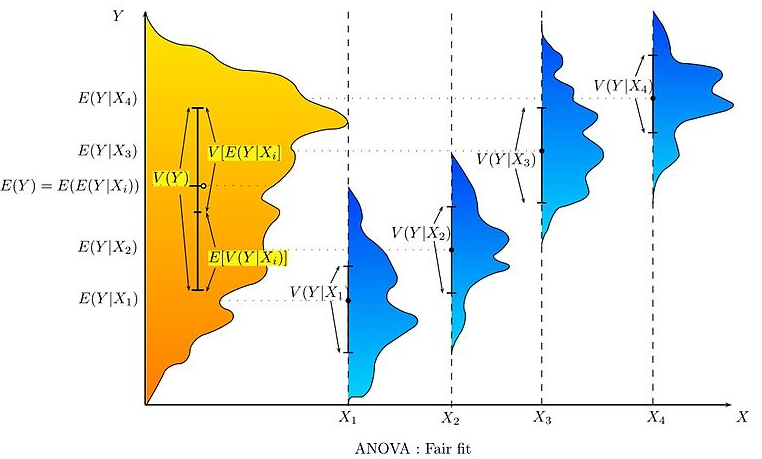
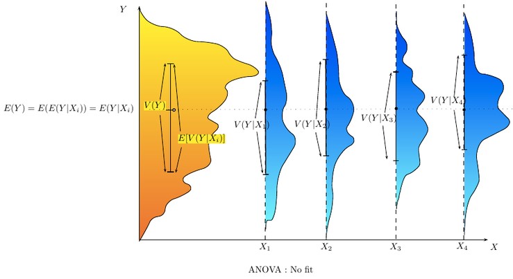
An attempt to explain the weight distribution by grouping dogs as (pet vs working breed) and (less athletic vs more athletic) would probably be somewhat more successful (fair fit). The heaviest show dogs are likely to be big strong working breeds, while breeds kept as pets tend to be smaller and thus lighter. As shown by the second illustration, the distributions have variances that are considerably smaller than in the first case, and the means are more reasonably distinguishable. However, the significant overlap of distributions, for example, means that we cannot reliably say that X1 and X2 are truly distinct (i.e., it is perhaps reasonably likely that splitting dogs according to the flip of a coin—by pure chance—might produce distributions that look similar).
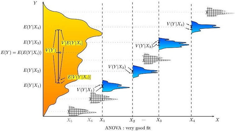
An attempt to explain weight by breed is likely to produce a very good fit. All Chihuahuas are light and all St Bernards are heavy. The difference in weights between Setters and Pointers does not justify separate breeds. The analysis of variance provides the formal tools to justify these intuitive judgments. A common use of the method is the analysis of experimental data or the development of models. The method has some advantages over correlation: not all of the data must be numeric and one result of the method is a judgment in the confidence in an explanatory relationship.
Classes of Models
There are three classes of models used in the analysis of variance, and these are outlined here.
- Fixed-effects models – The fixed-effects model (class I) of analysis of variance applies to situations in which the experimenter applies one or more treatments to the subjects of the experiment to see whether the response variable values change. This allows the experimenter to estimate the ranges of response variable values that the treatment would generate in the population as a whole.
- Random-effects models – Random effects model (class II) is used when the treatments are not fixed. This occurs when the various factor levels are sampled from a larger population.
- Mixed-effects models – A mixed-effects model (class III) contains experimental factors of both fixed and random-effects types, with appropriately different interpretations and analysis for the two types.
Defining fixed and random effects has proven elusive, with competing definitions arguably leading toward a linguistic quagmire.
Characteristics of ANOVA
ANOVA is used in the analysis of comparative experiments, those in which only the difference in outcomes is of interest. The statistical significance of the experiment is determined by a ratio of two variances. This ratio is independent of several possible alterations to the experimental observations.
Logic of ANOVA
The calculations of ANOVA can be characterized as computing a number of means and variances, dividing two variances and comparing the ratio to a handbook value to determine statistical significance. Calculating a treatment effect is then trivial, “the effect of any treatment is estimated by taking the difference between the mean of the observations which receive the treatment and the general mean
Partitioning of the sum of squares –
ANOVA uses traditional standardized terminology. The definitional equation of sample variance is ![]() , where the divisor is called the degrees of freedom (DF), the summation is called the sum of squares (SS), the result is called the mean square (MS) and the squared terms are deviations from the sample mean. ANOVA estimates 3 sample variances: a total variance based on all the observation deviations from the grand mean, an error variance based on all the observation deviations from their appropriate treatment means and a treatment variance
, where the divisor is called the degrees of freedom (DF), the summation is called the sum of squares (SS), the result is called the mean square (MS) and the squared terms are deviations from the sample mean. ANOVA estimates 3 sample variances: a total variance based on all the observation deviations from the grand mean, an error variance based on all the observation deviations from their appropriate treatment means and a treatment variance
The fundamental technique is a partitioning of the total sum of sqares SS into components related to the effects used in the model. For example, the model for a simplified ANOVA with one type of treatment at different levels.
![]()
The number of degrees of freedom DF can be partitioned in a similar way: one of these components (that for error) specifies a chi-squared distribution which describes the associated sum of squares, while the same is true for “treatments” if there is no treatment effect.
![]()
