A categorical variable is ordinal if there is a natural ordering of its possible categories. If there is no natural ordering, it is nominal.
Because it is not appropriate to perform arithmetic on the values of the variable, there are only a few possibilities for describing the variable, and these are all based on counting. First, you can count the number of categories. Many categorical variables such as Gender have only two categories. Others such as Region can have more than two categories. As you count the categories, you can also give the categories names, such as Male and Female.
Once you know the number of categories and their names, you can count the number of observations in each category (this is referred to as the count of categories). The resulting counts can be reported as “raw counts” or they can be transformed into percentages of totals. For example, if there are 1000 observations, you can report that there are 560 males and 440 females, or you can report that 56% of the observations are males and 44% are females.
A dummy variable is a variable with possible values 0 and 1. It equals 1 if the observation is in a particular category and 0 if it is not.
Categorical variables are used in two situations. The first is when a categorical variable has only two categories. A good example of this is a gender variable that has the two categories “male” and “female.” In this case only a single dummy variable is required, and you have the choice of assigning the 1s to either category. If the dummy variable is called Gender, you can code Gender as 1 for males and 0 for females, or you can code Gender as 1 for females and 0 for males. You just need to be consistent and specify explicitly which coding scheme you are using.
The other situation is when there are more than two categories. A good example of this is when you have quarterly time series data and you want to treat the quarter of the year as a categorical variable with four categories, 1 through 4. Then you can create four dummy variables, Q1 through Q4. For example, Q2 equals 1 for all second-quarter observations and 0 for all other observations. Although you can create four dummy variables, only three of them—any three—should be used in a regression equation.
A categorical variable that can take on exactly two values is termed a binary variable or dichotomous variable; an important special case is the Bernoulli variable. Categorical variables with more than two possible values are called polytomous variables; variables are often assumed to be polytomous unless otherwise specified. Discretization is treating continuous data as if it were categorical. Dichotomization is treating continuous data or polytomous variables as if they were binary variables. Regression analysis often treats category membership as a quantitative dummy variable.
Categorical variables represent a qualitative method of scoring data (i.e. represents categories or group membership). These can be included as independent variables in a regression analysis or as dependent variables in logistic regression or probit regression, but must be converted to quantitative data in order to be able to analyze the data. One does so through the use of coding systems. Analyses are conducted such that only g -1 (g being the number of groups) are coded. This minimizes redundancy while still representing the complete data set as no additional information would be gained from coding the total g groups: for example, when coding gender (where g = 2: male and female), if we only code females everyone left over would necessarily be males. In general, the group that one does not code for is the group of least interest.
There are three main coding systems typically used in the analysis of categorical variables in regression: dummy coding, effects coding, and contrast coding. The regression equation takes the form of Y = bX + a, where b is the slope and gives the weight empirically assigned to an explanator, X is the explanatory variable, and a is the Y-intercept, and these values take on different meanings based on the coding system used. The choice of coding system does not affect the F or R2 statistics. However, one chooses a coding system based on the comparison of interest since the interpretation of b values will vary.
Dummy Coding
Dummy coding is used when there is a control or comparison group in mind. One is therefore analyzing the data of one group in relation to the comparison group: a represents the mean of the control group and b is the difference between the mean of the experimental group and the mean of the control group. It is suggested that three criteria be met for specifying a suitable control group: the group should be a well-established group (e.g. should not be an “other” category), there should be a logical reason for selecting this group as a comparison (e.g. the group is anticipated to score highest on the dependent variable), and finally, the group’s sample size should be substantive and not small compared to the other groups.
In dummy coding, the reference group is assigned a value of 0 for each code variable, the group of interest for comparison to the reference group is assigned a value of 1 for its specified code variable, while all other groups are assigned 0 for that particular code variable.
The b values should be interpreted such that the experimental group is being compared against the control group. Therefore, yielding a negative b value would entail the experimental group have scored less than the control group on the dependent variable. To illustrate this, suppose that we are measuring optimism among several nationalities and we have decided that French people would serve as a useful control. If we are comparing them against Italians, and we observe a negative b value, this would suggest Italians obtain lower optimism scores on average.
The following table is an example of dummy coding with French as the control group and C1, C2, and C3 respectively being the codes for Italian, German, and Other (neither French nor Italian nor German):
| Nationality | C1 | C2 | C3 |
| French | 0 | 0 | 0 |
| Italian | 1 | 0 | 0 |
| German | 0 | 1 | 0 |
| Other | 0 | 0 | 1 |
Effects Coding
In the effects coding system, data are analyzed through comparing one group to all other groups. Unlike dummy coding, there is no control group. Rather, the comparison is being made at the mean of all groups combined (a is now the grand mean). Therefore, one is not looking for data in relation to another group but rather, one is seeking data in relation to the grand mean.
Effects coding can either be weighted or unweighted. Weighted effects coding is simply calculating a weighted grand mean, thus taking into account the sample size in each variable. This is most appropriate in situations where the sample is representative of the population in question. Unweighted effects coding is most appropriate in situations where differences in sample size are the result of incidental factors. The interpretation of b is different for each: in unweighted effects coding b is the difference between the mean of the experimental group and the grand mean, whereas in the weighted situation it is the mean of the experimental group minus the weighted grand mean.
In effects coding, we code the group of interest with a 1, just as we would for dummy coding. The principal difference is that we code −1 for the group we are least interested in. Since we continue to use a g – 1 coding scheme, it is in fact the −1 coded group that will not produce data, hence the fact that we are least interested in that group. A code of 0 is assigned to all other groups.
The b values should be interpreted such that the experimental group is being compared against the mean of all groups combined (or weighted grand mean in the case of weighted effects coding). Therefore, yielding a negative b value would entail the coded group as having scored less than the mean of all groups on the dependent variable. Using our previous example of optimism scores among nationalities, if the group of interest is Italians, observing a negative b value suggest they score obtain a lower optimism score.
The following table is an example of effects coding with Other as the group of least interest.
| Nationality | C1 | C2 | C3 |
| French | 0 | 0 | 1 |
| Italian | 1 | 0 | 0 |
| German | 0 | 1 | 0 |
| Other | −1 | −1 | −1 |
Example
Assume data pertaining to employment records of a sample of employees
| i | Sex | Merit Pay | i | Sex | Merit Pay |
| Bob | M | 9.6 | Tim | M | 6.0 |
| Paul | M | 8.3 | George | M | 1.1 |
| Mary | F | 4.2 | Alan | M | 9.2 |
| John | M | 8.8 | Lisa | F | 3.3 |
| Nancy | F | 2.1 | Anne | F | 2.7 |
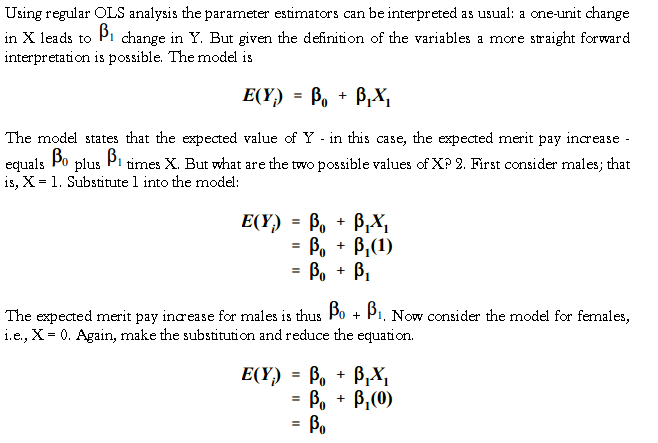
Here the dependent variable, Y, is merit pay increase measured in percent and the “independent” variable is sex which is quite obviously a nominal or categorical variable. Our goal is to use categorical variables to explain variation in Y, a quantitative dependent variable.
Step 1. We need to convert the categorical variable gender into a form that “makes sense” to regression analysis. One way to represent a categorical variable is to code the categories 0 and 1 as let X = 1 if sex is “male” 0 otherwise as Bob is scored “1” because he is male; Mary is 0.
Called dummy variables, data coded according this 0 and 1 scheme, are in a sense arbitrary but still have some desirable properties. A dummy variable, in other words, is a numerical representation of the categories of a nominal or ordinal variable. By creating X with scores of 1 and 0 we can transform the above table into a set of data that can be analyzed with regular regression. Here is what the “data matrix” would look like prior
| i | Sex | Merit Pay | i | Sex | Merit Pay |
| Bob | 1 | 9.6 | Tim | 1 | 6.0 |
| Paul | 1 | 8.3 | George | 1 | 1.1 |
| Mary | 0 | 4.2 | Alan | 1 | 9.2 |
| John | 1 | 8.8 | Lisa | 0 | 3.3 |
| Nancy | 0 | 2.1 | Anne | 0 | 2.7 |
Except for the first column, these data can be considered numeric: merit pay is measured in percent, while gender is “dummy” or “binary” variable with two values, 1 for “male” and 0 for “female.”
- We can use these numbers in formulas just like any data.
- Of course, there is something artificial about choosing 0 and 1, for why couldn’t we use 1 and 2 or 33 and 55.6 or any other pair of numbers?
- The answer is that we could. Using scores of 0 and 1, however, leads to particularly simple interpretations of the results of regression analysis.
Step 2 Interpretation Of Coefficients
If the categorical variable has K categories (e.g., region which might have K = 4 categories–North, South, Midwest, and West) one uses K – 1 dummy variables as seen later.
If we used other pairs of numbers, we would get the “correct” results but they would be hard to interpret.
