Multiple regression is an extension of simple linear regression. It is used when we want to predict the value of a variable based on the value of two or more other variables. The variable we want to predict is called the dependent variable (or sometimes, the outcome, target or criterion variable).
Nearly all real-world regression models involve multiple predictors, and basic descriptions of linear regression are often phrased in terms of the multiple linear regression, also known as multivariable linear regression.
Multiple regression also allows you to determine the overall fit of the model and the relative contribution of each of the predictors to the total variance explained. For example, you might want to know how much of the variation in exam performance can be explained by revision time, test anxiety, lecture attendance and gender “as a whole”, but also the “relative contribution” of each independent variable in explaining the variance.
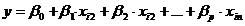
At the center of the multiple linear regression analysis is the task of fitting a single line through a scatter plot. More specifically the multiple linear regression fits a line through a multi-dimensional cloud of data points. The simplest form has one dependent and two independent variables, the general form of the multiple linear regression is defined as
for i = 1…n .
Sometimes the dependent variable is also called endogenous variable or prognostic variable. The independent variables are also called exogenous variables, predictor variables or regressors.
There are 3 major uses for Multiple Linear Regression Analysis – (1) causal analysis, (2) forecasting an effect, (3) trend forecasting. Other than correlation analysis, which focuses on the strength of the relationship between two or more variables, regression analysis assumes a dependence or causal relationship between one or more independent and one dependent variable.
Firstly, it might be used to identify the strength of the effect that the independent variables have on a dependent variable. Typical questions are what is the strength of relationship between dose and effect, sales and marketing spend, age and income.
Secondly, it can be used to forecast effects or impacts of changes. That is multiple linear regression analysis helps us to understand how much will the dependent variable change, when we change the independent variables. Typical questions are how much additional Y do I get for one additional unit X.
Thirdly, multiple linear regression analysis predicts trends and future values. The multiple linear regression analysis can be used to get point estimates. Typical questions are what will the price for gold be in 6 month from now? What is the total effort for a task X?
When selecting the model for the multiple linear regression analysis another important consideration is the model fit. Adding independent variables to a multiple linear regression model will always increase its statistical validity, because it will always explain a bit more variance (typically expressed as R²).
Example
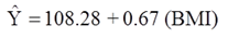
Suppose we want to assess the association between BMI and systolic blood pressure using data collected a study. A total of n=3,539 participants attended the exam, and their mean systolic blood pressure was 127.3 with a standard deviation of 19.0. The mean BMI in the sample was 28.2 with a standard deviation of 5.3. A simple linear regression analysis reveals the following:
| Independent Variable | Regression Coefficient | T | P-value |
| Intercept | 108.28 | 62.61 | 0.0001 |
| BMI | 0.67 | 11.06 | 0.0001 |
The simple linear regression model is:
Suppose we now want to assess whether age (a continuous variable, measured in years), male gender (yes/no), and treatment for hypertension (yes/no) are potential confounders, and if so, appropriately account for these using multiple linear regression analysis. For analytic purposes, treatment for hypertension is coded as 1=yes and 0=no. Gender is coded as 1=male and 0=female. A multiple regression analysis reveals the following:
| Independent Variable | Regression Coefficient | T | P-value |
| Intercept | 68.15 | 26.33 | 0.0001 |
| BMI | 0.58 | 10.30 | 0.0001 |
| Age | 0.65 | 20.22 | 0.0001 |
| Male gender | 0.94 | 1.58 | 0.1133 |
| Treatment for hypertension | 6.44 | 9.74 | 0.0001 |
The multiple regression model is

Notice that the association between BMI and systolic blood pressure is smaller (0.58 versus 0.67) after adjustment for age, gender and treatment for hypertension. BMI remains statistically significantly associated with systolic blood pressure (p=0.0001), but the magnitude of the association is lower after adjustment. The regression coefficient decreases by 13%.
Using the informal rule (i.e., a change in the coefficient in either direction by 10% or more), we meet the criteria for confounding. Thus, part of the association between BMI and systolic blood pressure is explained by age, gender and treatment for hypertension.
This also suggests a useful way of identifying confounding. Typically, we try to establish the association between a primary risk factor and a given outcome after adjusting for one or more other risk factors. One useful strategy is to use multiple regression models to examine the association between the primary risk factor and the outcome before and after including possible confounding factors. If the inclusion of a possible confounding variable in the model causes the association between the primary risk factor and the outcome to change by 10% or more, then the additional variable is a confounder.
