It is a statistical process for estimating the relationships among variables. It includes many techniques for modeling and analyzing several variables, when the focus is on the relationship between a dependent variable and one or more independent variables (or ‘predictors’). More specifically, regression analysis helps one understand how the typical value of the dependent variable (or ‘criterion variable’) changes when any one of the independent variables is varied, while the other independent variables are held fixed.
Regression analysis is widely used for prediction and forecasting. Many techniques for carrying out regression analysis have been developed. Familiar methods such as linear regression and ordinary least squares regression are parametric, in that the regression function is defined in terms of a finite number of unknown parameters that are estimated from the data. Nonparametric regression refers to techniques that allow the regression function to lie in a specified set of functions, which may be infinite-dimensional.
The performance of regression analysis methods in practice depends on the form of the data generating process, and how it relates to the regression approach being used. Since the true form of the data-generating process is generally not known, regression analysis often depends to some extent on making assumptions about this process. These assumptions are sometimes testable if a sufficient quantity of data is available.
In a multiple relationship, called multiple regression, two or more independent variables are used to predict one dependent variable. For example, an educator may wish to investigate the relationship between a student’s success in college and factors such as the number of hours devoted to studying, the student’s GPA, and the student’s high school background. This type of study involves several variables.
Simple relationships can also be positive or negative. A positive relationship exists when both variables increase or decrease at the same time. For instance, a person’s height and weight are related; and the relationship is positive, since the taller a person is, generally, the more the person weighs. In a negative relationship, as one variable increases, the other variable decreases, and vice versa.
Simple Regression
In simple regression studies, the researcher collects data on two numerical or quantitative variables to see whether a relationship exists between the variables. For example, if a researcher wishes to see whether there is a relationship between number of hours of study and test scores on an exam, she must select a random sample of students, determine the hours each studied, and obtain their grades on the exam.
The two variables for this study are called the independent variable and the dependent variable. The independent variable is the variable in regression that can be controlled or manipulated.
The independent and dependent variables can be plotted on a graph called a scatter plot. The independent variable x is plotted on the horizontal axis, and the dependent variable y is plotted on the vertical axis.
Scatter Diagram
It displays multiple XY coordinate data points represent the relationship between two different variables on X and Y-axis. It is also called as correlation chart. It depicts the relationship strength between an independent variable on the vertical axis and a dependent variable on the horizontal axis. It enables strategizing on how to control the effect of the relationship on the process. It is also called scatter plots, X-Y graphs or correlation charts.
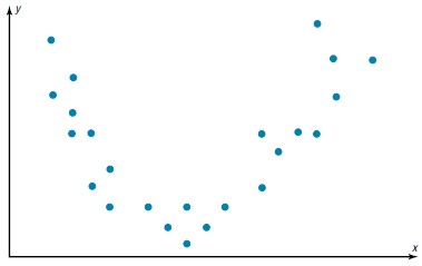
It is used when two variables are related or evaluating paired continuous data. It is also helpful to identify potential root causes of a problem by relating two variables. The tighter the data points along the line, the stronger the relationship amongst them and the direction of the line indicates whether the relationship is positive or negative. The degree of association between the two variables is calculated by the correlation coefficient. If the points show no significant clustering, there is probably no correlation.
Correlation Coefficient
Statisticians use a measure called the correlation coefficient to determine the strength of the linear relationship between two variables. There are several types of correlation coefficients.
The correlation coefficient computed from the sample data measures the strength and direction of a linear relationship between two variables. The symbol for the sample correlation coefficient is r. The symbol for the population correlation coefficient is r (Greek letter rho).
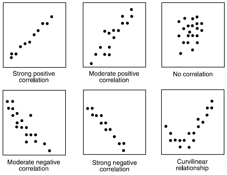
The range of the correlation coefficient is from -1 to +1. If there is a strong positive linear relationship between the variables, the value of r will be close to +1. If there is a strong negative linear relationship between the variables, the value of r will be close to -1. When there is no linear relationship between the variables or only a weak relationship, the value of r will be close to 0.
Formula for the Correlation Coefficient r
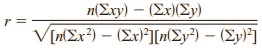
where n is the number of data pairs.
Population Correlation Coefficient
The population correlation coefficient is computed from taking all possible (x, y) pairs; it is designated by the Greek letter r (rho). The sample correlation coefficient can then be used as an estimator of r if the following assumptions are valid.
- The variables x and y are linearly related.
- The variables are random variables.
- The two variables have a bivariate normal distribution.
A biviarate normal distribution means that for the pairs of (x, y) data values, the corresponding y values have a bell-shaped distribution for any given x value, and the x values for any given y value have a bell-shaped distribution.
Formally defined, the population correlation coefficient r is the correlation computed by using all possible pairs of data values ( x, y) taken from a population.
Significance of the Correlation coefficients
In hypothesis testing, one of these is true:
H0: r equals 0 – This null hypothesis means that there is no correlation between the x and y variables in the population.
H1: r not equals 0 – This alternative hypothesis means that there is a significant correlation between the variables in the population.
When the null hypothesis is rejected at a specific level, it means that there is a significant difference between the value of r and 0. When the null hypothesis is not rejected, it means that the value of r is not significantly different from 0 (zero) and is probably due to chance.
Several methods can be used to test the significance of the correlation coefficient like the t test, as
![]()
with degrees of freedom equal to n – 2.
Although hypothesis tests can be one-tailed, most hypotheses involving the correlation coefficient are two-tailed. Recall that r represents the population correlation coefficient.
Standard Error of Estimate
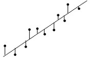
The standard error of the estimate is a measure of the accuracy of predictions made with a regression line. The standard error of the estimate is a measure of the accuracy of predictions.
S represents the average distance that the observed values fall from the regression line. Conveniently, it tells you how wrong the regression model is on average using the units of the response variable. Smaller values are better because it indicates that the observations are closer to the fitted line. S becomes smaller when the data points are closer to the line.
The standard error for the estimate is calculated by the following formula:
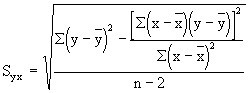
The formula may look formidable, but we already have calculated all of the components except for squaring the ![]() This approximate value for the standard error of the estimate tells us the accuracy to expect from our prediction.
This approximate value for the standard error of the estimate tells us the accuracy to expect from our prediction.
