Regression analysis is used in the practice of Six Sigma to forecast the change in the dependent variable in your process. You use regression analysis to describe the relationship between the predictor variables – the variable x factors you will change and the response variables or y outputs of the process.
When the input and output variables are both continuous and to see a relationship between the two variables, regression and correlation are used. Determining how the predicted or dependent variable (the response variable, the variable to be estimated) reacts to the variations of the predicator or independent variable (the variable that explains the change) involves first to determine any relationship between them and it’s importance. Regression analysis builds a mathematical model that helps making predictions about the impact of variable variations.
Usually, there is more than one independent variable causing variations of a dependent variable like changes in the volume of cars sold depends on the price of the cars, the gas mileage, the warranty, etc. But the importance of all these factors in the variation of the dependent variable (the number of cars sold) is disproportional. Hence, project team should concentrate on one important factor instead of analyzing all the competing factors.
Simple Linear Regression
In it, the prediction of scores on one variable is done from the scores on a second variable. The variable to predict is called the criterion variable and is referred to as Y. The variable to base predictions on is called the predictor variable and is referred to as X. When there is only one predictor variable, the prediction method is called simple regression. In simple linear regression, the predictions of Y when plotted as a function of X form a straight line. Simple linear regression gives you a line of best fit, which is a line going through the center of the plotted data on a scatter diagram. The simple regression formula enables you to make predictions about what you’re going to get out of the process. For each y value, you’re looking for one x value.
As an example, data for X and Y are listed below and having a positive relationship between X and Y. For predicting Y from X, the higher the value of X, the higher prediction of Y.
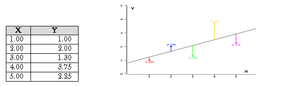
Linear regression consists of finding the best-fitting straight line through the points. The best-fitting line is called a regression line. The diagonal line in the figure is the regression line and consists of the predicted score on Y for each possible value of X. The vertical lines from the points to the regression line represent the errors of prediction. As the line from 1.00 is very near the regression line; its error of prediction is small and similarly for the line from 1.75 is much higher than the regression line and therefore its error of prediction is large.
The error of prediction for a point is the value of the point minus the predicted value (the value on the line). The below table shows the predicted values (Y’) and the errors of prediction (Y-Y’) like, for the first point has a Y of 1.00 and a predicted Y (called Y’) of 1.21 hence, its error of prediction is -0.21.
| X | Y | Y’ | Y-Y’ | (Y-Y’)2 |
| 1.00 | 1.00 | 1.210 | -0.210 | 0.044 |
| 2.00 | 2.00 | 1.635 | 0.365 | 0.133 |
| 3.00 | 1.30 | 2.060 | -0.760 | 0.578 |
| 4.00 | 3.75 | 2.485 | 1.265 | 1.600 |
| 5.00 | 2.25 | 2.910 | -0.660 | 0.436 |
The most commonly-used criterion for the best-fitting line is the line that minimizes the sum of the squared errors of prediction. That is the criterion that was used to find the line in the figure. The last column in the above table shows the squared errors of prediction. The sum of the squared errors of prediction shown in the above table is lower than it would be for any other regression line.
The regression equation is calculated with the mathematical equation for a straight line as y = b0+ b1 X where, b0 is the y intercept when X= 0 and b1 is the slope of the line with the assumption that for any given value of X, the observed value of Y varies in a random manner and possesses a normal probability distribution. For calculations are based on the statistics, assuming MX is the mean of X, MY is the mean of Y, sX is the standard deviation of X, sY is the standard deviation of Y, and r is the correlation between X and Y, a sample data is as
| MX | MY | sX | sY | r |
| 3 | 2.06 | 1.581 | 1.072 | 0.627 |
The slope (b) can be calculated as b = r sY/sX and the intercept (A) as A = MY – bMX. For the above data, b = (0.627)(1.072)/1.581 = 0.425 and A = 2.06 – (0.425)(3) = 0.785. The calculations have all been shown in terms of sample statistics rather than population parameters. The formulas are the same but need the usage of the parameter values for means, standard deviations, and the correlation.
Least Squares Method
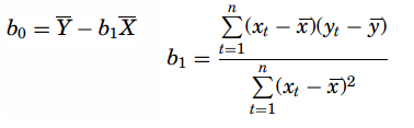
In this method, for computing the values of b1 and b0, the vertical distance between each point and the line called the error of prediction is used. The line that generates the smallest error of predictions will be the least squares regression line. The values of b1 and b0 are computed as
The P-value is determined by referring to a t-distribution with n-2 degrees of freedom.
Multiple Linear Regression
Multiple linear regression expands on the simple linear regression model to allow for more than one independent or predictor variable. The general form for the equation is y = b0+ b1x + … bn+ e where, (b0,b1,b2…) are the coefficients and are referred to as partial regression coefficients. The equation may be interpreted as the amount of change in y for each unit increase in x (variable) when all other xs are held constant. The hypotheses for multiple regression are Ho:b1=b2= … =bn Ha:b1≠ 0 for at least one i.
In the case of a multiple lineal regression, multiple y’s can come into play. For example, if you’re only comparing height and weight, that would be a simple linear regression. However, if you compare height, age, and gender and then plot that against weight, you would actually have three different factors. You’d be analyzing three different multiple lineal regressions.
It is an extension of linear regression to more than one independent variable so a higher proportion of the variation in Y may be explained as first-order linear model

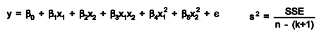
And second-order linear model
R2 the multiple coefficient of determination has values in the interval 0<=R2<=1
| Source | DF | SS | MS |
| Regression | k | SSR | MSR=SSR/k |
| Error | n-(k+1) | SSE | MSE=SSE[n-(k+1)] |
| Total | n-1 | Total SS |
