Dividend Discount Model
The dividend discount model (DDM) is one of the most basic absolute valuation models. The dividend model calculates the “true” value of a firm based on the dividends the company pays to its shareholders.
This model values the shares at the present value of future dividend payments. A share is worth the present value of all future dividends. As it values shares on the actual cash flows received by investors, it is theoretically the most correct valuation model.
Expressed mathematically
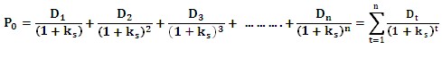
Where:
However for applying this method:
- The company should be paying dividends.
- The dividend pay-out ratio should be stable and predictable.
The companies that pay stable and predictable dividends are typically mature blue-chip companies in mature and well-developed industries. These type of companies are often best suited for this type of valuation method. When the earnings per share are consistently growing and the dividends are also growing at the same rate, the trend is a consistent one and forecasting for future periods would be easier.
One problem with dividend discount model is that long term forecasting is difficult, and the valuation is very sensitive to the inputs used: the discount rate and any growth rates in particular.
This is true for any Discounted Cash Flow (DCF) model, but a dividend discount model adds an extra dimension to the difficulty in forecasting by requiring forecasts of dividends, which means anticipating the dividend policy a company will adopt. As with other DCF models, the discount rate is most likely to be calculated using CAPM.
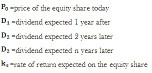
Gordon Growth Model
The Gordon Growth Model is a form of the Dividend Discount model. It determines the intrinsic value of a stock, based on a future series of dividends that grow at a constant rate. Given a dividend per share that is payable in one year, and the assumption that the dividend grows at a constant rate in perpetuity, the model solves for the present value of the infinite series of future dividends.
Mathematically expressed

Where:
D = Expected dividend per share one year from now
Ks = Required rate of return for equity investor
g = Growth rate in dividends (in perpetuity)
As the model simplistically assumes a constant growth rate, it is generally only used for mature companies (or broad market indices) with low to moderate growth rates.
6.3.3 Free cash flow Model
The Free Cash Flow (FCF) to the firm is the cash generated by operations, which is attributed to all providers of capital in the firm’s capital structure. This includes debt providers as well as equity.
Calculating the FCF is done by taking earnings before interest and taxes and adjusting for the tax rate, then adding depreciation and taking away capital expenditure, minus change in working capital and minus changes in other assets. Here is the actual formula:
FCF = EBIT (1-T) + depreciation – CAPEX – ∆working capital – ∆ any other assets
Where:
EBIT = earnings before interest and taxes
T= tax rate
CAPEX = capital expenditure
In the valuation method this cash flow is taken before the interest payments to debt holders in order to value the total firm. Only factoring in equity, for example, would provide the growing value to equity holders.
Discounting any stream of cash flows requires a discount rate, and in this case it is the cost of financing projects at the firm. The weighted average cost of capital (WACC) is used for this discount rate. The operating free cash flow is then discounted at this cost of capital rate using three potential growth scenarios; no growth, constant growth and changing growth rate.
No Growth
To find the value of the firm, discount the FCF by the WACC. This discounts the cash flows that are expected to continue for as long as a reasonable forecasting model exists.
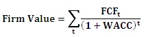
Where:
FCFt= the operating free cash flows in period t
WACC = weighted average cost of capital
For an estimate for the value of the firm’s equity, subtract the market value of the firm’s debt.
Constant Growth
In a more mature company it is more appropriate to include a constant growth rate in the calculation. To calculate the value, take the FCF of next period and discount it at WACC minus the long-term constant growth rate of the OFCF.
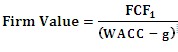
Where:
FCFt = operating free cash flow
g = expected growth rate in FCF
Multiple Growth Periods
Assuming the firm is about to see more than one growth stage, the calculation is a combination of each of these stages. Using the supernormal dividend growth model for the calculation, the analyst needs to predict the higher-than-normal growth and the expected duration of such activity. After this high growth, the firm might be expected to go back into a normal steady growth into perpetuity.
Comparing this to the company’s current stock price can be a valid way of determining the company’s intrinsic value. The total current value of the firm’s debt is subtracted to get the value of the equity. Dividing the equity value by common shares outstanding would provide the value of equity per share. This value can then be compared to the market price to see if it is over- or undervalued.
Relative Valuation Model
Relative valuation methods for valuing a stock are summarized as follows.
Price/Earnings (P/E) Ratio: The most commonly used relationship between stock prices and earnings is the price/earnings (P/E) ratio, computed by dividing the market price of the stock by its earnings per share. The P/E ratio indicates the multiple that an investor is willing to pay for a unit of company’s earnings. There are two widely held assumptions regarding P/E ratios. The first is that stocks in the same industry have similar P/E ratios; the second is that stocks tend to trade within a range of P/E ratios. The P/E ratio shows the number of times that a stock’s price is trading relative to its earnings, and because stock prices fluctuate, so do their ratios. Rising P/E ratios generally are linked to higher stock prices. Another use of the ratio is to divide a company’s market price by its projected earnings per share. If the market price of a stock is $30 and its projected earnings per share are $4, the P/E ratio is 7.5. If analysts think that the appropriate ratio for companies in this industry is 9, then this stock is undervalued.
Using P/E ratios to value stocks has several weaknesses. Determining the appropriate P/E ratio is subjective, and P/E ratios can fluctuate considerably. Theoretically, if earnings per share increase, the stock price should rise so that the P/E ratio stays the same. In reality, this situation does not happen often. P/E ratios can be volatile and fluctuate considerably, making this a difficult indicator to read over short periods of time. Longer term, P/E ratios are more accurate in determining whether a company is over- or undervalued.
Another major weakness is the use of earnings per share (EPS). By definition, earnings per share include extraordinary gains and losses that are nonrecurring. The inclusion of a one-time gain overstates earnings per share and causes the P/E ratio to be lower. Consequently, the stock might appear to be undervalued.
Another stumbling block is the use of historical earnings versus future earnings, which is discussed further in Table 9–3. Because of these weaknesses in the use of the P/E ratio, short-term results as to the valuation of a stock could be misleading. Over longer time periods, these aberrations even out, and the P/E ratio becomes a more meaningful indicator of a company’s stock value.
Price/Earnings Growth (PEG) Ratio: The price/earnings growth ratio is the company’s P/E ratio divided by the company’s estimated future growth rate in earnings per share. The price/earnings growth (PEG) ratio indicates how much an investor pays for the growth of a company. For example, a company with an estimated growth rate of 16 percent and a P/E ratio of 20 has a PEG ratio of 1.25 (20 / 16). For growth rates that are less than the P/E ratio, the value of the PEG ratio is greater than 1.0. A growth rate that exceeds the P/E ratio results in a value that is less than 1.0.
The lower the ratio, the greater is the potential increase in stock price, assuming that the company can grow at its projected growth rate. A stock generally is perceived to be undervalued if the growth rate of the company exceeds its P/E ratio. A high PEG ratio implies that the stock is overvalued. Put another way, the lower the PEG ratio, the less an investor pays for estimated future earnings. If the estimated earnings growth rate is inaccurate, the PEG ratio will be unreliable as an indicator of value.
Historical earnings show a company’s actual earnings, but the past is not always accurately projected into the future. The use of historical earnings results in higher P/E ratios than using forward earnings during periods of earnings growth. The opposite is also true: In periods of declining earnings growth, the use of historical earnings results in lower P/E ratios than use of forward earnings. Forward earnings are only estimates that are determined subjectively by financial analysts.
Price–to–Book Value Ratio: Some investors look for stocks whose market prices are trading below their book values. The book value per share is computed by deducting the total liabilities from total assets and then dividing this number by the number of shares outstanding. The use of book value per share as a valuation tool is not compelling because many factors overstate or understate the book value of a stock.
For example, buildings and real estate are recorded at historical costs (original purchase prices), although market prices can be significantly higher or lower, thereby distorting the book value per share. A low value suggests that the stock is undervalued, and a high value indicates the opposite. As with the P/E and PEG ratios, what differentiates a stock from being overvalued and undervalued is determined subjectively.
Investors looking for value stocks would place more emphasis on finding stocks whose book values are greater than their market values. Value stocks tend to have lower P/E ratios, lower growth rates, and lower price–to–book value ratios than growth stocks do.
Price-to-Sales Ratio: The price-to-sales ratio indicates how much an investor is willing to pay for every rupee of sales of that company. The ratio is computed by dividing the market price of the stock by the sales per share. This ratio measures the valuation of a company on the basis of sales rather than earnings. You should compare the company’s price-to-sales ratio with that of the industry to determine whether the company is trading at a compelling valuation to its sales base. A low price-to-sales ratio indicates that the company has room to expand its sales and, therefore, its earnings.
Price–to–Cash Flow Ratio: Earnings are an important determinant of a company’s value, but the company’s cash position is another important way to assess value. A company’s statement of changes in cash is a good starting point for assessing cash flow. Cash flow is computed by adding noncash charges, such as depreciation and amortization, to net income (after-tax income). Cash flow per share is computed by dividing the cash flow by the number of common shares outstanding.
Cash flow per share is considered by many analysts to be a better yardstick of valuation than earnings per share. The amount of cash flow a company can generate indicates the company’s capability to finance its own growth without having to resort to external funding sources.
The price–to–cash flow ratio is similar to the P/E ratio except that the cash flow per share is substituted for earnings per share. In other words, the market price of the stock is divided by the cash flow per share to equal the price–to–cash flow ratio. As with the P/E ratio, the lower the price–to–cash flow ratio, the more compelling is the value of the company. The advantage of using cash flow over earnings per share is that a company can have negative earnings per share but positive cash flow per share.
SOTP Valuation
Sum-of-the-parts (SOTP) or “break-up” analysis provides a range of values for a company’s equity by summing the value of its individual business segments to arrive at the total enterprise value (EV). Equity value is then calculated by deducting net debt and other non-operating adjustments.
For a company with different business segments, each segment is valued using ranges of trading and transaction multiples appropriate for that particular segment. Relevant multiples used for valuation, depending on the individual segment’s growth and profitability, may include revenue, EBITDA, EBIT, and net income. A DCF analysis for certain segments may also be a useful tool when forecasted segment results are available or estimable.
SOTP analysis is used to value a company with business segments in different industries that have different valuation characteristics.
The methodology can be summarized as follows.
- Gather segment-level data from any of the following sources:
- Investor presentations
- Corporate web sites
- Research reports
- Latest annual report
- Moody’s company profiles
- Spread LTM and, to the extent possible, projected financial data for each business segment
- Typical financial metrics used include EBITDA, EBIT, and net income
- The SOTP financial information should equal the consolidated financial information for the entire company
- As necessary, an “other” category may be used, but care should be taken to determine the nature of this category in order to assess multiples, value, etc.
- Allocate corporate overhead to divisions based on percent of revenues, EBIT, or industry norms for each segment. It is also acceptable to value overhead as a standalone item
- If depreciation and amortization are not provided by segment, allocate to divisions using methodologies that may include percent of assets, revenues, EBIT, or industry norms for each segment
- Use your judgment to the extent necessary
- Determine an appropriate range of multiples for each business segment by applying metrics and multiples which are most relevant for each business segment
- Use either trading or transaction comps, as appropriate, for each industry to determine the appropriate range
- Use a range of multiples, not point estimates
- To the extent overhead was not allocated; apply blended multiples to determine the “negative value” of overhead. Since this may create misleading values for the individual segments, allocating overhead is preferable, assuming there is sufficient data
- DCF valuations may be useful for certain business segments
- Sum the values of each business segment, offset by corporate overhead, if appropriate. The result is an aggregate EV range for the consolidated company
- Deduct net debt and add/subtract other non-operating / financial items from the EV range to determine a range of equity values.
- Divide by the sum of diluted shares outstanding to arrive at a range of equity values per diluted share. Be sure to include any in-the-money options and convertible securities.
- Other considerations.
- Minority interest could be attributable to a single segment or may have components from all segments. If attributable to a single segment, be sure to make note of it in the valuation analysis
- Similarly, certain liabilities may be attributable to one or more segments, or may be entirely separate
- Interpreting the Analysis: Compare the range of results to current trading levels to determine whether the company is overvalued or undervalued. Also, compare results to any of the following metrics and look for consistency with the calculated range.
- 52-week high and low
- Comparable company’s analysis
- Wall Street research
Apply for Equity Research Certification Now!!
http://www.vskills.in/certification/Certified-Equity-Research-Analyst
