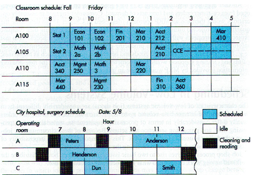
Loading refers to the assignment of jobs to processing (work) centers and to various machines in the work centers. Problems arise when two or more jobs are to be processed and there are a number of work centers capable of performing the required work. Managers often seek an arrangement that will minimize processing and setup costs, minimize idle time among work centers, or minimize job completion time.
Loading involves specific tasks being allocated to specific teams, individuals, or facilities. Once there is adequate capacity, loading is used to assign each worker the task they can perform best. In the case of a machine or a facility, loading is used to assign the process to the one that can carry it out most efficiently.
There are two approaches used to load work centers:
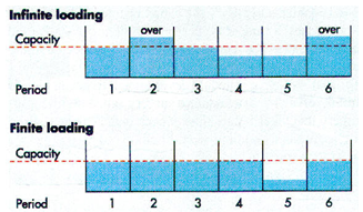
- infinite – The infinite loading method assigns work to work centers without that center’s capacity being taken into account. With the infinite loading approach, priority rules are suitable. This means that jobs are loaded at work centers according to the predefined priority rule. This approach is known as vertical loading. If an organization has limited capacity and uses infinite loading, it may have to increase capacity through overtime, subcontracting, or expansion.
- finite – With finite loading, the start and stop time of each job at the work center is projected.
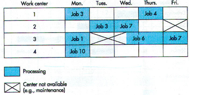
Gantt Chart
Gantt charts are used as visual aid for loading and scheduling purposes. The name was derived from Henry Gantt in the early 1900s. The purpose of Gantt charts is to organize and clarify the actual or intended use of resources in a time framework. In most cases, a time scale is represented horizontally, and resources to be scheduled are listed vertically. The use of resources is reflected in the body of the chart.
There are a number of different types of Gantt charts. Two of the most commonly used are the load chart and the schedule chart.
Load Chart
A load chart depicts the loading and idle times for a group of machines or a list of departments. The chart shows when certain jobs are scheduled to start and finish, and where to expect idle time. If all centers perform the same kind of work, the manager might want to free one center for a long job or a rush order.
Two different approaches are used to load work centers, infinite loading and finite loading. Infinite loading assign jobs to work centers without regard to the capacity of the work center. One possible result of infinite loading is the formation of queues in some work centers. Finite loading projects actual job starting and stopping times at each work center, taking into account the capacities of each work center and the processing times of jobs, so that capacity is not exceeded. Schedules based on finite loading may have to be updated often, perhaps daily, due to processing delays at work centers and the addition of new jobs or cancellation of current jobs. The following diagram illustrates these two approaches.
Loading can be done in various ways. Vertical loading refers to loading jobs at a work center job by job, usually according to some priority criterion. Vertical loading does not consider the work center’s capacity (i.e., infinite loading). With vertical loading, a manager may need to make some response to overloaded work centers. Among the possible responses are shifting work to other periods or other centers, working overtime, or contracting out a portion of the work. In contrast, horizontal loading involves loading the job that has the highest priority on all work centers it will require, then the job with the next highest priority, and so on. Horizontal loading is based on finite loading.
One possible result of horizontal loading is keeping jobs waiting at a work center even though the center is idle, so the center will be ready to process a higher priority job that is expected to arrive shortly. That would not happen with vertical loading; the work center would be fully loaded, although a higher priority job would have to wait if it arrived while the work center was busy. So, the horizontal loading takes a more global approach to scheduling, while vertical loading uses a local approach.
Which approach is better? That depends on various factors: the relative costs of keeping higher priority jobs waiting, the cost of having work centers idle, the number of jobs, the number of work centers, the potential for processing disruptions, the potential for new jobs and job cancellations, and so on.
Schedule Chart
There are two general approaches to scheduling: forward scheduling and backward scheduling. Forward scheduling means scheduling ahead from a point in time; backward scheduling means scheduling backward from a due date. Forward scheduling is used if the issue is “How long will it take to complete this job?” Backward scheduling would be used if the issue is ” When is the latest job can be started and still be completed by the due date?” A manager often uses a schedule chart to monitor the progress of jobs. A typical schedule chart is illustrated below for a landscaping job.
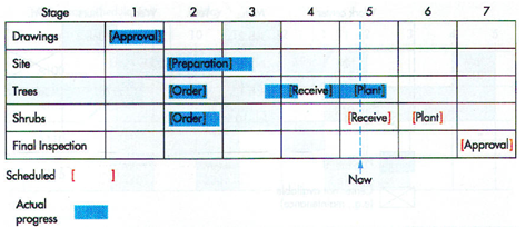
The chart shows planned and actual starting and finishing times for the five stages of the job. The chart indicates that approval and ordering of trees and shrubs was on schedule. The site preparation was a little behind schedule The trees were received earlier than expected, and planting is ahead of schedule. However, the shrubs have not yet been received. The chart indicates some slack between scheduled receipt of shrubs and shrub planting, so if the shrubs arrive by the end of the week, it appears the schedule can still be met.
The Gantt charts possess certain limitations. The chief one is the need to repeatedly update a chart to keep it current. In addition, a chart does not directly reveal costs associated with alternative loading. Finally, a job’s processing time may vary depending on the work center; certain work stations or work centers may be capable of processing some jobs faster than other stations.
Input / Output Control
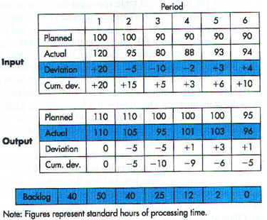
Input / output (I/O) control refers to monitoring the work flow and queue length at work centers. The purpose is to manage work flow so that queues and waiting times are kept under control. A simple example of I/O control is the use of stoplights on some expressway on ramps. These regulate the flow of entering traffic according to the current volume of expressway traffic. The following figure illustrates an input / output report for a work center. The deviation in each period are determined by subtracting “planned” from “actual”. The backlog for each period is determined by subtracting the “actual output” from the “actual input” and adjusting the backlog from the previous period by that amount.
Assignment Method of Linear Programming
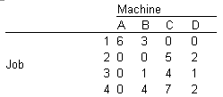
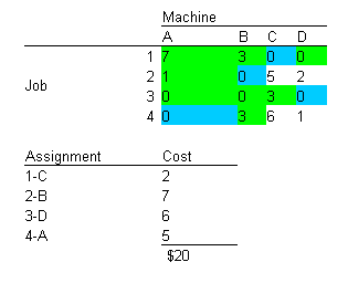
The following table illustrates a typical problem, where four jobs are to be assigned to four machines
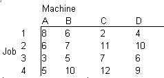
The numbers in the body of the table represent the value or cost associated with each job machine combination. In this case, the numbers represent costs. If the problem involved minimizing the cost for job 1 alone, it would clearly be assigned to machine C. For n machines, there are n! different possibilities. For 12 jobs, there would be 479 million different matches! A simple solution method for one-to-one matching is called the Hungarian method to identify the lowest-cost solution. The method assumes that every machine is capable of handling every job, and that the costs or values associated with each assignment combination are known and fixed. When profits instead of costs are involved, the profits can be converted into relative costs by subtracting every number in the table from the largest number and then processing as in a minimization problem. In addition, specific combinations can be avoided by assigning a relatively high cost to that combination. The basic procedure of the Hungarian method is:
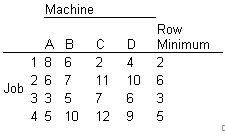
- Row reduction: Subtract the smallest number in each row from every number in the row.
- Column reduction: Subtract the smallest number in each column of the new table from every number in the column.
- Test whether an optimum assignment can be made by determining the minimum number of lines (horizontal or vertical) needed to cross out all zeros. If the number of lines equals the number of rows, an optimum assignment is possible. In that case, go to step 6. Otherwise, go on to step 4.
- If the number of lines is less than the number of rows, modify the table in this way:
- Subtract the smallest uncovered number from every uncovered number in the table.
- Add the smallest uncovered number to the numbers at intersections of cross-out lines.
- Numbers crossed out but not at intersections of cross-out lines carry over unchanged to the next table.
- Repeat steps 3 and 4 until an optimal table is obtained.
- Make the assignments. Begin with rows and columns with only one zero. Match items that have zeros, using only one match for each row and each column. Eliminate both the row and the column after the match.
Example
Determine the optimum assignment of jobs to machines for the following data.
Solution
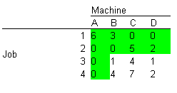
Subtract the smallest number in each row from every number in the row, and enter the result in a new table. The result of this row reduction is
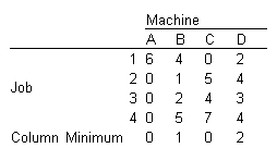
Subtract the smallest number in each column from every number in the column, and enter the results in a new table. The result of this column reduction is
Determine the minimum number of lines (in green background) needed to cross out all zeros. (Try to cross out as many zeros as possible when drawing lines.)
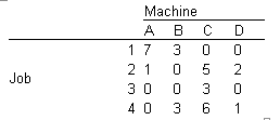
Since only three lines are needed to cross out all zeros and the table has four rows, this is not the optimum. Subtract the smallest value that hasn’t been crossed out (in this case, 1) from every number that hasn’t been crossed out, and add it to numbers that are at the intersections of covering lines. The results are
Determine the minimum number of lines needed to cross out all zeros (four). Since this equals the number of rows, you can make the optimum assignment.
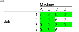
Make assignments: Start with rows and columns with only one zero. Match jobs with machines that have a zero cost.
Sequencing
Sequencing is concerned with determining both the order in which jobs are processed at various work centers and the order in which jobs are processed at individual workstations within the work centers. When work centers are heavily loaded, the order of processing can be very important in terms of costs associated with jobs waiting for processing and in terms of idle time at the work centers.
Priority rules are simple heuristics used to select the order in which the jobs will be processed. Some of the most common are listed below.
- FCFS (first come, first served): Jobs are processed in the order in which they arrive at a machine or work center.
- Last Come First Served (LCFS) – The first job loaded to a machine in a work center will be the last one that arrives.
- SPT (shortest processing time): Jobs are processed according to processing time at a machine or work center, shortest job first.
- EDD (earliest due date): Jobs are processed according to due date, earliest due date first.
- CR (critical ratio): Jobs are processed according to smallest ratio of time remaining until due date to processing time remaining.
- S/O (slack per operation): Jobs are processed according to average slack time (time until due date minus remaining time to process). Compute by dividing slack time by number of remaining operations, including the current one.
- Rush: Emergency or preferred customers first.
The rules generally rest on the following assumptions.
- The set of jobs is known; no new jobs arrive after processing begins; and no jobs are canceled.
- Setup time is independent of processing sequence.
- Setup time is deterministic.
- Processing time is deterministic rather than variable.
- There will be no interruptions in processing such as machine breakdowns, accidents, or work illness.
Job time usually includes setup and processing times. Jobs that require similar setups can lead to reduced setup times, if the sequencing rule takes this into account (the rules here do not).
Due dates may be the result of delivery times promised to customers, MRP processing, or managerial decisions. They are subject to revision and must be kept current to give meaning to sequencing choices. It should be noted that due date associated with all rules except S/O and CR are for the operation about to be performed; due dates for S/O and CR are typically final due dates for orders rather than intermediate, departmental deadlines.
The priority rules can be classified as either local or global. Local rules take into account information pertaining only to a single workstation; global rules take into account information pertaining to multiple workstations. FCFS, SPT, and EDD are local rules; CR and S/O are global rules. Rush can be either local or global. Global rules require more effort than local rules. A major complication in global sequencing is that not all jobs require the same processing or even the same order of processing. As a result, the set of jobs is different for different workstations. Local rules are particularly useful for bottleneck operations, but they are not limited to those situations. The effectiveness of any given sequence is frequently judged in terms of one or more performance measures. The most frequently used performance measures are:
Job flow time: Job flow time is the length of time that begins when a job arrives at the shop, workstation, or work center, and ends when it leaves the shop, workstation, or work center. It includes not only actual processing time but also any time waiting to be processed, transportation time between operations, and any waiting time related to equipment breakdowns, unavailable parts, quality problems, and so on. The average flow time for a group of jobs is equal to the total flow time for the jobs divided by the number of jobs.
Job lateness: This is the length of time the job completion date is expected to exceed the date the job was due or promised to a customer. If we only record differences for jobs with completion times that exceed due dates, and assign zeros to jobs that are early, the term we use to refer to that is job tardiness.
Makespan: Makespan is the total time needed to complete a group of jobs. It is the length of time between the start of the first job in the group and the completion of the last job in the group.
Average number of jobs: Jobs that are in a shop are considered to be work-in-process inventory. If the jobs represent equal amounts of inventory, the average number of jobs will also reflect the average work-in-process inventory. The average work-in-process for a group of jobs can be computed using the following formula:
Example
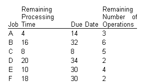
Processing times (including setup times) and due dates for six jobs waiting to be processed at a work center are given in the following table. Determine the sequence of jobs, the average flow time, average days late, and average number of jobs at the work center, for each of these rules:
- FCFS
- SPT
- EDD
- CR
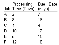
Assume jobs arrived in the order shown.
Solution
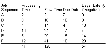
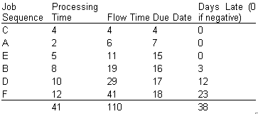
The FCFS sequence is simple A-B-C-D-E-F. The measures of effectiveness are (see table below):
Average flow time: 120/6 = 20 days.
Average tardiness: 54/6 = 9 days.
The makespan is 41 days. Average number of jobs at the work center: 120/41=2.93.
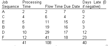
Using the SPT rule, the job sequence is A-C-E-B-D-F (see the following table). The resulting values for the three measures of effectiveness are
Average flow time: 108/6 = 18 days.
Average tardiness: 40/6 = 6.67 days.
The makespan is 41 days. Average number of jobs at the work center: 108/41=2.63.
Using earliest due date as the election criterion, the job sequence is C-A-E-B-D-F. The measures of effectiveness are (see table):
Average flow time: 110/6 = 18.33 days.
Average tardiness: 38/6 = 6.33 days.
The makespan is 41 days. Average number of jobs at the work center: 110/41=2.68.
Using the critical ratio we find:
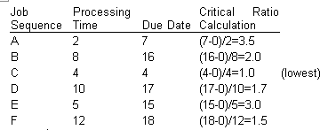
At day 4 [C completed], the critical ratios are:
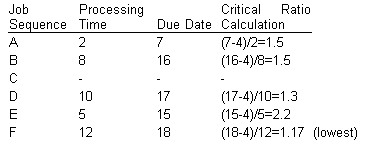
At day 16 [C and F completed], the critical ratios are:
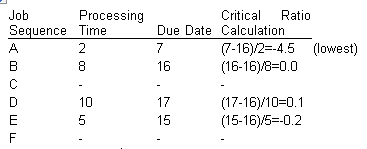
At day 18 [C, F, and A completed], the critical ratios are:
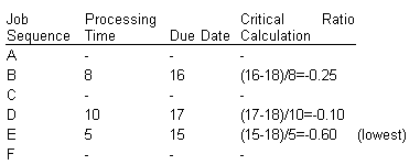
At day 23 [C, F, A, and E completed], the critical ratios are:
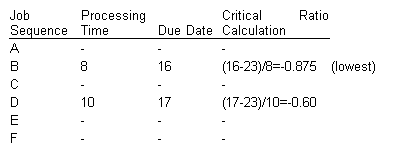
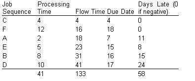
The job sequence is C-F-A-E-B-D, and the resulting values for the measures of effectiveness are:
Average flow time: 133/6 = 22.17 days.
Average tardiness: 58/6 = 9.67 days.
The makespan is 41 days. Average number of jobs at the work center: 133/41=3.24.
The results of these four rules are summarized below.
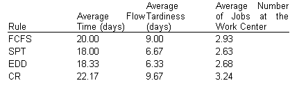
Generally speaking, SPT is superior in terms of minimizing flow time and, hence, in terms of minimizing the average number of jobs at the work center and completion time. The FCFS rule and the CR rule turn out to be the least effective of the rules.
The primary limitation of FCFS rule is that long jobs will tend to delay their jobs. However, for service systems in which customers are directly involved, the FCFS rule is by far the dominant priority rule, mainly because of the inherent fairness but also because of the inability to obtain realistic estimates of processing time for individual jobs. The FCFS rule also has the advantage of simplicity. If other measures are important when there is high customer contact, companies may adopt the strategy of moving processing to the “backroom” so they don’t necessarily have to follow FCFS.
Because the SPT rule always results in the lowest (i.e., optimal) average completion (flow) time, it can result in lower in-process inventories. And, because it often provides the lowest (optimal) average tardiness, it can result in better customer levels. Finally, since it always involves a lower average number of jobs at the work center, there tends to be less congestion in the work area. SPT also minimizes downstream idle time. However, due dates are often uppermost in managers’ minds, so they may not use SPT, because it doesn’t incorporate due dates. The major disadvantage of the SPT rule is that it tends to make long jobs wait, perhaps for rather long times (especially if new, shorter jobs are continuously added to the system). Various modifications may be used in an effort to avoid this. For example, after waiting for a given time period, any remaining jobs are automatically moved to the head of the line. This is known as the truncated SPT rule.
The EDD rule directly addresses due dates and usually minimizes lateness. Although it has intuitive appeal, its main limitation is that it does not take processing time into account. One possible consequence is that it can result in some jobs waiting a long time, which adds to both in-process inventories and shop congestion.
The CR rule is easy to use and has intuitive appeal. Although it had the poorest showing in the example for all three measures, it usually does quite well in terms of minimizing job tardiness. Therefore, if jab tardiness is important the CR rule might be the best choice among the rules.
Example
Use S/O (slack per operation) rule to schedule the following jobs. Note that processing time includes the time remaining for the current and subsequent operations. In addition, you will need to know the number of operations remaining, including the current one.
Solution
Determine the difference between the due date and the processing time for each operation. Divide the amount by the number of remaining operations, and rank them from low to high. This yields the sequence of jobs:
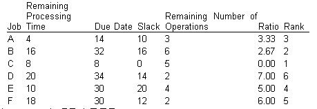
The indicated sequence is C-B-A-E-F-D.
Using the S/O rule, the designated job sequence may change after any given operation, so it is important to re-evaluate the sequence after each operation. Note that any of the previously mentioned priority rules could be used on a station-by-station basis for this situation; the only difference is that the S/O approach incorporates downstream information in arriving at a job sequence.
Sequencing Jobs Through Two Work Centers
Johnson’s rule is a technique that managers can use to minimize the makespan for a group of jobs to be processed on two machines or at two successive work centers (sometimes referred to as a two-machine flow shop). It also minimizes the total idle time at the work centers. For the technique to work, several conditions must be satisfied:
- Job time (including setup and processing) must be known and constant for each job at each work center.
- Job times must be independent of the job sequence.
- All jobs must follow the same two-step work sequence.
- Job priorities cannot be used.
- All units in a job must be completed at the first work center before the job moves on to the second work center.
Determination of the optimum sequence involves these steps:
- List the jobs and their times at each work center.
- Select the job with the shortest time. If the shortest time is at the first work center, schedule that job first; if the time is at the second work center, schedule the job last. Break ties arbitrarily.
- Eliminate the job and its time from further consideration.
- Repeat steps 2 and 3, working toward the center of the sequence until all jobs have been scheduled.
When significant idle time at the second work center occurs, job splitting at the first center just priori to the occurrence of idle time may alleviate some of it and also shorten throughput time.
Example
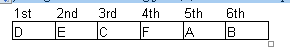
A group of six jobs is to be processed through a two-machine flow shop. The first operation involves cleaning and the second involves painting. Determine a sequence that will minimize the total completion time for this group of jobs. Processing times are as follows:
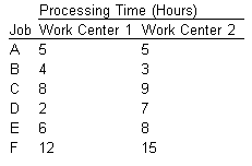
Solution
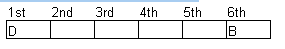
Select the job with the shortest processing time. It is job D with a time of 2 hours.
Since the time is at the first center, schedule job D first. Eliminate job D from further consideration.
Job B has the next shortest time. Since it is at the second work center, schedule it last and eliminate job B from further consideration. We now have
The remaining jobs and their times are
Note that there is a tie for the shortest remaining time: job A has the same time at each work center. It makes no difference, then, whether we place it toward the beginning or the end of the sequence. Suppose it is placed arbitrarily toward the end. We now have
The shortest remaining time is 6 hours for job E at work center 1. Thus, schedule that job toward the beginning of the sequence (after job D). Thus,
Job C has the shortest time of the remaining two jobs. Since it is for the first work center, place it third in the sequence. Finally, assign the remaining job (F) to the fourth position and the result is
One way to determine the throughput time and idle times at the work centers is to construct a chart:
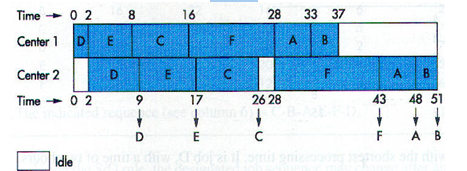
Thus, the group of jobs will take 51 hours to complete. The second work center will wait 2 hours for its first job and also wait 2 hours after finishing job C. Center 1 will be finished in 37 hours. Of course, idle periods at the beginning or end of the sequence could be used to do other jobs or for maintenance or setup/teardown activities.
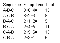
Sequence Jobs When Setup Times Are Sequence-Dependent
The simplest way to determine which sequence will result in the lowest total setup time is to list each possible sequence and determine its total setup time. As the number of jobs increases, a manager would use a computer to generate the list and identify the best alternative(s).
Example
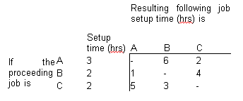
Solution
B-A-C.
Important Guidelines
- Setting realistic due dates.
- Focusing on bottleneck operations: First, try to increase the capacity of the operations. If that is not possible or feasible, schedule the bottleneck operations first, and then schedule the non-bottleneck operations around the bottleneck operations.
- Considering lot splitting for large jobs. This probably works best when there are relatively large differences in job times.
