Apache Hive is a data warehouse infrastructure built on top of Hadoop for providing data summarization, query, and analysis. While initially developed by Facebook, Apache Hive is now used and developed by other companies such as Netflix. Amazon maintains a software fork of Apache Hive that is included in Amazon Elastic MapReduce on Amazon Web Services.
Apache Hive supports analysis of large datasets stored in Hadoop’s HDFS and compatible file systems such as Amazon S3 filesystem. The primary responsibility is to provide data summarization, query and analysis. Hive is built for data mining applications. It provides an SQL-like language called HiveQL with schema on read and transparently converts queries to map/reduce, Apache Tez and Spark jobs. All three execution engines can run in Hadoop YARN. To accelerate queries, it provides indexes, including bitmap indexes.
By default, Hive stores metadata in an embedded Apache Derby database, and other client/server databases like MySQL can optionally be used.
Currently, there are four file formats supported in Hive, which are TEXTFILE, SEQUENCEFILE, ORC and RCFILE. Apache Parquet can be read via plugin in versions later than 0.10 and natively starting at 0.13.
The Apache Hive data warehouse software facilitates querying and managing large datasets residing in distributed storage. Built on top of Apache Hadoop, it provides
- Tools to enable easy data extract/transform/load (ETL)
- A mechanism to impose structure on a variety of data formats
- Access to files stored either directly in Apache HDFS or in other data storage systems such as Apache HBase.
- Query execution via MapReduce
Hive defines a simple SQL-like query language, called QL, that enables users familiar with SQL to query the data. At the same time, this language also allows programmers who are familiar with the MapReduce framework to be able to plug in their custom mappers and reducers to perform more sophisticated analysis that may not be supported by the built-in capabilities of the language. QL can also be extended with custom scalar functions (UDF’s), aggregations (UDAF’s), and table functions (UDTF’s). Hive does not mandate read or written data be in the “Hive format” — there is no such thing. Hive works equally well on Thrift, control delimited, or your specialized data formats.
Hive is not designed for OLTP workloads and does not offer real-time queries or row-level updates. It is best used for batch jobs over large sets of append-only data (like web logs). What Hive values most are scalability (scale out with more machines added dynamically to the Hadoop cluster), extensibility (with MapReduce framework and UDF/UDAF/UDTF), fault-tolerance, and loose-coupling with its input formats.
Components of Hive include HCatalog and WebHCat.
- HCatalog is a component of Hive. It is a table and storage management layer for Hadoop that enables users with different data processing tools — including Pig and MapReduce — to more easily read and write data on the grid.
- WebHCat provides a service that you can use to run Hadoop MapReduce (or YARN), Pig, Hive jobs or perform Hive metadata operations using an HTTP (REST style) interface.
Installation
Start by downloading the most recent stable release of Hive from one of the Apache download mirrors. Next you need to unpack the tarball. This will result in the creation of a subdirectory named hive-x.y.z (where x.y.z is the release number):
$ tar -xzvf hive-x.y.z.tar.gz
Set the environment variable HIVE_HOME to point to the installation directory:
$ cd hive-x.y.z
$ export HIVE_HOME={{pwd}}
Finally, add $HIVE_HOME/bin to your PATH:
$ export PATH=$HIVE_HOME/bin:$PATH
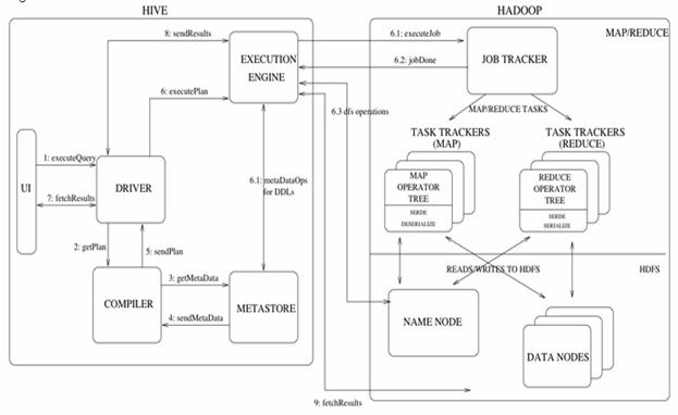
Figure above shows the major components of Hive and its interactions with Hadoop. As shown in that figure, the main components of Hive are:
- UI – The user interface for users to submit queries and other operations to the system. As of 2011 the system had a command line interface and a web based GUI was being developed.
- Driver – The component which receives the queries. This component implements the notion of session handles and provides execute and fetch APIs modeled on JDBC/ODBC interfaces.
- Compiler – The component that parses the query, does semantic analysis on the different query blocks and query expressions and eventually generates an execution plan with the help of the table and partition metadata looked up from the metastore.
- Metastore – The component that stores all the structure information of the various tables and partitions in the warehouse including column and column type information, the serializers and deserializers necessary to read and write data and the corresponding HDFS files where the data is stored.
- Execution Engine – The component which executes the execution plan created by the compiler. The plan is a DAG of stages. The execution engine manages the dependencies between these different stages of the plan and executes these stages on the appropriate system components.
Figure above also shows how a typical query flows through the system. The UI calls the execute interface to the Driver (step 1 in Figure). The Driver creates a session handle for the query and sends the query to the compiler to generate an execution plan (step 2). The compiler gets the necessary metadata from the metastore (steps 3 and 4). This metadata is used to typecheck the expressions in the query tree as well as to prune partitions based on query predicates. The plan generated by the compiler (step 5) is a DAG of stages with each stage being either a map/reduce job, a metadata operation or an operation on HDFS. For map/reduce stages, the plan contains map operator trees (operator trees that are executed on the mappers) and a reduce operator tree (for operations that need reducers). The execution engine submits these stages to appropriate components (steps 6, 6.1, 6.2 and 6.3). In each task (mapper/reducer) the deserializer associated with the table or intermediate outputs is used to read the rows from HDFS files and these are passed through the associated operator tree. Once the output is generated, it is written to a temporary HDFS file though the serializer (this happens in the mapper in case the operation does not need a reduce). The temporary files are used to provide data to subsequent map/reduce stages of the plan. For DML operations the final temporary file is moved to the table’s location. This scheme is used to ensure that dirty data is not read (file rename being an atomic operation in HDFS). For queries, the contents of the temporary file are read by the execution engine directly from HDFS as part of the fetch call from the Driver (steps 7, 8 and 9).
Hive Data Model
Data in Hive is organized into:
- Tables – These are analogous to Tables in Relational Databases. Tables can be filtered, projected, joined and unioned. Additionally all the data of a table is stored in a directory in HDFS. Hive also supports the notion of external tables wherein a table can be created on prexisting files or directories in HDFS by providing the appropriate location to the table creation DDL. The rows in a table are organized into typed columns similar to Relational Databases.
- Partitions – Each Table can have one or more partition keys which determine how the data is stored, for example a table T with a date partition column ds had files with data for a particular date stored in the <table location>/ds=<date> directory in HDFS. Partitions allow the system to prune data to be inspected based on query predicates, for example a query that is interested in rows from T that satisfy the predicate T.ds = ‘2008-09-01’ would only have to look at files in <table location>/ds=2008-09-01/ directory in HDFS.
- Buckets – Data in each partition may in turn be divided into Buckets based on the hash of a column in the table. Each bucket is stored as a file in the partition directory. Bucketing allows the system to efficiently evaluate queries that depend on a sample of data (these are queries that use the SAMPLE clause on the table).
Apart from primitive column types (integers, floating point numbers, generic strings, dates and booleans), Hive also supports arrays and maps. Additionally, users can compose their own types programmatically from any of the primitives, collections or other user-defined types. The typing system is closely tied to the SerDe (Serailization/Deserialization) and object inspector interfaces. User can create their own types by implementing their own object inspectors, and using these object inspectors they can create their own SerDes to serialize and deserialize their data into HDFS files). These two interfaces provide the necessary hooks to extend the capabilities of Hive when it comes to understanding other data formats and richer types. Builtin object inspectors like ListObjectInspector, StructObjectInspector and MapObjectInspector provide the necessary primitives to compose richer types in an extensible manner. For maps (associative arrays) and arrays useful builtin functions like size and index operators are provided. The dotted notation is used to navigate nested types, for example a.b.c = 1 looks at field c of field b of type a and compares that with 1.
Metastore
The Metastore provides two important but often overlooked features of a data warehouse: data abstraction and data discovery. Without the data abstractions provided in Hive, a user has to provide information about data formats, extractors and loaders along with the query. In Hive, this information is given during table creation and reused every time the table is referenced. This is very similar to the traditional warehousing systems. The second functionality, data discovery, enables users to discover and explore relevant and specific data in the warehouse. Other tools can be built using this metadata to expose and possibly enhance the information about the data and its availability. Hive accomplishes both of these features by providing a metadata repository that is tightly integrated with the Hive query processing system so that data and metadata are in sync.
Metadata Objects
- Database – is a namespace for tables. It can be used as an administrative unit in the future. The database ‘default’ is used for tables with no user-supplied database name.
- Table – Metadata for a table contains list of columns, owner, storage and SerDe information. It can also contain any user-supplied key and value data. Storage information includes location of the underlying data, file inout and output formats and bucketing information. SerDe metadata includes the implementation class of serializer and deserializer and any supporting information required by the implementation. All of this information can be provided during creation of the table.
- Partition – Each partition can have its own columns and SerDe and storage information. This facilitates schema changes without affecting older partitions.
Metastore Architecture – Metastore is an object store with a database or file backed store. The database backed store is implemented using an object-relational mapping (ORM) solution called the DataNucleus. The prime motivation for storing this in a relational database is queriability of metadata. Some disadvantages of using a separate data store for metadata instead of using HDFS are synchronization and scalability issues. Additionally there is no clear way to implement an object store on top of HDFS due to lack of random updates to files. This, coupled with the advantages of queriability of a relational store, made our approach a sensible one.
The metastore can be configured to be used in a couple of ways: remote and embedded. In remote mode, the metastore is a Thrift service. This mode is useful for non-Java clients. In embedded mode, the Hive client directly connects to an underlying metastore using JDBC. This mode is useful because it avoids another system that needs to be maintained and monitored. Both of these modes can co-exist. (Update: Local metastore is a third possibility.
Metastore Interface – Metastore provides a Thrift interface to manipulate and query Hive metadata. Thrift provides bindings in many popular languages. Third party tools can use this interface to integrate Hive metadata into other business metadata repositories.
Hive Query Language
HiveQL is an SQL-like query language for Hive. It mostly mimics SQL syntax for creation of tables, loading data into tables and querying the tables. HiveQL also allows users to embed their custom map-reduce scripts. These scripts can be written in any language using a simple row-based streaming interface – read rows from standard input and write out rows to standard output. This flexibility comes at a cost of a performance hit caused by converting rows from and to strings. However, we have seen that users do not mind this given that they can implement their scripts in the language of their choice. Another feature unique to HiveQL is multi-table insert. In this construct, users can perform multiple queries on the same input data using a single HiveQL query. Hive optimizes these queries to share the scan of the input data, thus increasing the throughput of these queries several orders of magnitude. We omit more details due to lack of space.
Logging
Hive uses log4j for logging. These logs are not emitted to the standard output by default but are instead captured to a log file specified by Hive’s log4j properties file. By default Hive will use hive-log4j.default in the conf/ directory of the Hive installation which writes out logs to /tmp/<userid>/hive.log and uses the WARN level. It is often desirable to emit the logs to the standard output and/or change the logging level for debugging purposes. These can be done from the command line as follows:
$HIVE_HOME/bin/hive –hiveconf hive.root.logger=INFO,console
hive.root.logger specifies the logging level as well as the log destination. Specifying console as the target sends the logs to the standard error (instead of the log file).
