Functions are prewritten formulas that perform certain types of calculations automatically. The syntax or rules of structure for entering all functions is
Function name (arguments1, argument2…)
The functions name identifies the type of calculations to be performed. Most functions require that we enter one or more arguments following the function name. An argument is the data the function uses to perform the calculation. The type of data the function requires depends upon the type of calculation being performed.
Using Arguments
Arguments are values that a function uses to perform operations or calculations. The type of argument a function uses is specific to the function. Common arguments that are used within functions include numeric values, text values, cell references, ranges of cells, names, labels, and nested functions.
Using Functions Wizard to create formulae
Following steps are taken to create formulae
- Click the cell in which we want to enter the formula.
- To start the formula with the function, in insert menu click function.
- Type function name or select by selecting “All” in select by category drop down list
- Click the function we want to add to the formula.
- Enter the arguments.
- When we complete the formula, press ENTER.
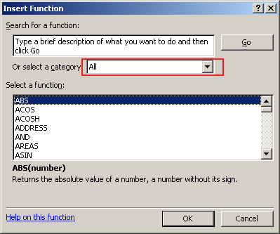
Insert function dialog box
Using names in formulas
You can use the labels of columns and rows on a worksheet to refer to the cells within those columns and rows. Or you can create descriptive names to represent cells, ranges of cells, formulas, or constant values. Labels can be used in formulas that refer to data on the same worksheet; if you want to represent a range on another worksheet, use a name.
A defined name in a formula can make it easier to understand the purpose of the formula. For example, the formula =SUM(FirstQuarterSales) might be easier to identify than =SUM(C20:C30).
Names are available to any sheet. For example, if the name ProjectedSales refers to the range A20:A30 on the first worksheet in a workbook, you can use the name ProjectedSales on any other sheet in the same workbook to refer to range A20:A30 on the first worksheet.
Names can also be used to represent formulas or values that do not change (constants). For example, you can use the name SalesTax to represent the sales tax amount (such as 6.2 percent) applied to sales transactions.
You can also link to a defined name in another workbook, or define a name that refers to cells in another workbook. For example, the formula =SUM(Sales.xls!ProjectedSales) refers to the named range ProjectedSales in the workbook named Sales By default, names use absolute cell references.
Guidelines for names
- The first character of a name must be a letter or an underscore character. Remaining characters in the name can be letters, numbers, periods, and underscore characters.
- Names cannot be the same as a cell reference, such as Z$100 or R1C1.
- More than one word be used but spaces are not allowed. Underscore characters and periods may be used as word separators— for example, Sales_Tax or First.Quarter.
- A name can contain up to 255 characters.
Names can contain uppercase and lowercase letters. Microsoft Excel does not distinguish between uppercase and lowercase characters in names. For example, if you have created the name Sales and then create another name called SALES in the same workbook, the second name will replace the first one.
Logical Functions
A Logical function is a function that tests, or evaluates, whether a condition in the workbook is true or false. The condition is usually entered as an expression. For example, the expression A1 = 10 would be true if cell At contains the value 10; otherwise, the expression is false.
A Logical function is a function that tests, or evaluates, whether a condition in the workbook is true or false. The condition is usually entered as an expression. For example, the expression A1 = 10 would be true if cell At contains the value 10; otherwise, the expression is false.
A conditional test is an equation that compares two items. These items can be numbers, functions, formulae, labels or logical values. A conditional test must include at least one logical operator. The result of a conditional test is either TRUE or FALSE.
The IF function
Returns one value if a condition we specify evaluates to TRUE and another value if it evaluates to FALSE. Use IF to conduct conditional tests on values and formulas.
IF (logical_test, value_if_true, value_if_false)
Logical_test is any value or expression that can be evaluated to TRUE or FALSE. For example, A10=100 is a logical expression; if the value in cell A10 is equal to 100, the expression evaluates to TRUE. Otherwise, the expression evaluates to FALSE. This argument can use any comparison calculation operator.
Value_if_true is the value that is returned if logical_test is TRUE. For example, if this argument is the text string “Within budget” and the logical_test argument evaluates to TRUE, then the IF function displays the text “Within budget”. If logical_test is TRUE and value_if_true is blank, this argument returns 0 (zero). To display the word TRUE, use the logical value TRUE for this argument. Value_if_true can be another formula.
Value_if_false is the value that is returned if logical_test is FALSE. For example, if this argument is the text string “Over budget” and the logical_test argument evaluates to FALSE, then the IF function displays the text “Over budget”. If logical_test is FALSE and value_if_false is omitted, (that is, after value_if_true, there is no comma), then the logical value FALSE is returned. If logical_test is FALSE and value_if_false is blank (that is, after value_if_true, there is a comma followed by the closing parenthesis), then the value 0 (zero) is returned. Value_if_false can be another formula.
Some points to be kept in mind while working with if function
- Up to seven IF functions can be nested as value_if_true and value_if_false arguments to construct more elaborate tests. See the following last example.
- When the value_if_true and value_if_false arguments are evaluated, IF returns the value returned by those statements.
- If any of the arguments to IF are arrays, every element of the array is evaluated when the IF statement is carried out.
Examples
On a budget sheet, cell A10 contains a formula to calculate the current budget. If the result of the formula in A10 is less than or equal to 100, then the following function displays “Within budget”. Otherwise, the function displays “Over budget”.
IF (A10<=100,”Within budget”,”Over budget”)
In the following example, if the value in cell A10 is 100, then logical_test is TRUE, and the total value for the range B5:B15 is calculated. Otherwise, logical_test is FALSE, and empty text (“”) is returned that blanks the cell that contains the IF function.
IF (A10=100,SUM (B5:B15),””)
Suppose an expense worksheet contains in B2:B4 the following data for “Actual Expenses” for January, February, and March: 1500, 500, 500. C2:C4 contains the following data for “Predicted Expenses” for the same periods: 900, 900, 925.
We can write a formula to check whether we are over budget for a particular month, generating text for a message with the following formulas
IF (B2>C2,”Over Budget”, ”OK”) equals “Over Budget”
IF (B3>C3,”Over Budget”, ”OK”) equals “OK”
Suppose we want to assign letter grades to numbers referenced by the name Average Score. See the following table. We can use the following nested IF function
| If Average Score is | Then return |
| Greater than 89 | A |
| From 80 to 89 | B |
| From 70 to 79 | C |
| From 60 to 69 | D |
| Less than 60 | F |
IF (Average Score>89,”A”, IF (Average Score>79,”B”,
IF (Average Score>69,”C”,
IF(Average Score>59,”D”,”F”))))
In the preceding example, the second IF statement is also the value_if_false argument to the first IF statement. Similarly, the third IF statement is the value_if_false argument to the second IF statement. For example, if the first logical_test (Average>89) is TRUE, “A” is returned. If the first logical_test is FALSE, the second IF statement is evaluated, and so on.
Nested IF statements
Sometimes your problem may be so involved that you cannot solve it by using just the techniques you have met so far. An extremely useful feature is the ability to nest IF functions (put one inside another). You can nest up to seven IF functions as long as the number of characters in your formula does not exceed the maximum number of characters that can be entered in a cell.
There is not a single general form but the following is typical:
=IF( condition1,value1,IF( condition2,value2,value3 ))
AND, OR and NOT
When building up a conditional test you sometimes need quite complicated conditions. These three functions can help to simplify the job. The functions AND and OR can take up to 30 logical arguments whereas NOT has only one argument.
General forms:
=AND(logical1,logical2,…,logical30 )
=OR(logical1,logical2,…,logical30 )
=NOT(logical1 )
The arguments for the functions can be
- conditional tests
- references to cells containing logical values
- arrays of logical values
AND
- If all the arguments in an AND function are true, the result is TRUE .
- If one or more arguments are false, the result is FALSE.
OR
- If at least one of the arguments in an OR function is true, the result is TRUE.
- If all the arguments in an OR function are false, the result is FALSE.
NOT
- This function negates a condition.
- If the argument in a NOT function is false, the result is TRUE.
- If the argument in a NOT function is true, the result is FALSE.
A few very simple examples follow
| Formula | Result |
| =AND(5>3,80<96) | TRUE |
| =AND(2*24<67,7<0.34,4*4=2*8) | FALSE |
| =OR(4*4=8*2,56>297) | TRUE |
| =OR(2=3,3=4,4=5) | FALSE |
| =NOT(5<3) | TRUE |
| =NOT(6=6) | FALSE |
| Function | Description |
| AND | Returns TRUE if all of its arguments are TRUE |
| FALSE | Returns the logical value FALSE |
| IF | Specifies a logical test to perform |
| IFERROR | Returns a value you specify if a formula evaluates to an error; otherwise, returns the result of the formula |
| NOT | Reverses the logic of its argument |
| OR | Returns TRUE if any argument is TRUE |
| TRUE | Returns the logical value TRUE |
Statistical functions
Excel provides a great deal of assistance when it comes to analysing statistical data. There are several built-in functions. In addition, the Analysis ToolPak can be used, which is an add-in module with a collection of functions and tools that enable you to produce rank-and-percentile tables, perform regression analysis, apply Fourier transformations to data, and so on.
The COUNT Function
Counts the number of cells that contain numbers and numbers within the list of arguments. Its usage is
COUNT (value1, value2…)
Value1, value2, … are 1 to 30 arguments that can contain or refer to a variety of different types of data, but only numbers are counted.
Arguments that are numbers, dates, or text representations of numbers are counted; arguments that are error values or text that cannot be translated into numbers are ignored.
The MAX Function
Returns the largest value in a set of values. Its usage is
MAX (number1, number2…)
Number1, number2… are 1 to 30 numbers for which you want to find the maximum value.
You can specify arguments that are numbers, empty cells, logical values, or text representations of numbers. Arguments that are error values or text that cannot be translated into numbers cause errors. If the arguments contain no numbers, MAX returns 0 (zero). Example
If A1:A5 contains the numbers 10, 7, 9, 27, and 2, then
MAX (A1:A5) equals 27
MAX (A1:A5, 30) equals 30
The MIN Function
Returns the smallest number in a set of values. Its usage is
MIN (number1, number2…)
Number1, number2… are 1 to 30 numbers for which you want to find the minimum value.
You can specify arguments that are numbers, empty cells, logical values, or text representations of numbers. Arguments that are error values or text that cannot be translated into numbers cause errors. If the arguments contain no numbers, MIN returns 0.
Example if A1:A5 contains the numbers 10, 7, 9, 27, and 2, then
MIN (A1:A5) equals 2
MIN (A1:A5, 0) equals 0
The AVERAGE Function
In the above example we have calculated the average of the values lying between B3 cell to B6, with the formula
=Average (B3:B6)
Date and Time Functions
The TODAY() Function and the NOW() Function – The TODAY function returns the serial number of today’s date based on your system clock and does not include the time. The NOW function returns the serial number of today’s date and includes the time.
In Excel, dates are sorted based on the serial number of the date, instead of on the displayed number. Therefore, when you sort dates in Excel, you may not receive the results you expect.
For example, if you sort a series of dates that are displayed in the mmmm date format (so that only the month is displayed), the months are not sorted alphabetically. Instead, the dates are sorted based on their underlying date serial number.
Because serial numbers are also used in date and time comparisons, actual results may be different than what you expect (based on the displayed values).
For example, when you use the NOW function to compare a date with the current date, as in the formula
=IF(NOW()=DATEVALUE(“10/1/92”),TRUE,FALSE)
the formula returns FALSE, even if the current date is 10/1/92; it returns TRUE only when the date is 10/1/92 12:00:00 a.m. If you are comparing two dates in a formula, and you do not have to have the time included in the result, you can work around this behavior by using the TODAY function instead:
=IF(TODAY()=DATEVALUE(“10/1/92”),TRUE,FALSE)
To find the number of days between now and a date sometime in the future, use the following formula
=”mm/dd/yy”-NOW()
where “mm/dd/yy” is the future date. Use the General format to format the cell that contains the formula.
Calculate Elapsed Time
When you subtract the contents of one cell from another to find the amount of time elapsed between them, the result is a serial number that represents the elapsed hours, minutes, and seconds. To make this number easier to read, use the h:mm time format in the cell that contains the result.
In the following example, if cells C2 and D2 contain the formula =B2-A2, and cell C2 is formatted in the General format, the cell displays a decimal number (in this case, 0.53125, the serial number representation of 12 hours and 45 minutes).
A1: Start Time B1: End Time C1: Difference D1: Difference
(General) (h:mm)
A2: 6:30 AM B2: 7:15 PM C2: 0.53125 D2: 12:45
If midnight falls between your start time and end time, you must account for the 24-hour time difference. You can do this by adding the number 1, which represents one 24-hour period. For example, you might set up the following table, which allows for time spans beyond midnight.
A1: Start Time B1: End Time C1: Difference D1: Difference
(General) (h:mm)
A2: 7:45 PM B2: 10:30 AM C2: 0.614583333 D2: 14:45
To set up this table, type the following formula in cells C2 and D2:
=B2-A2+IF(A2>B2,1)
If you want to correctly display a time greater than 24 hours, you can use the 37:30:55 built-in format. If you want to use a custom format instead, you must enclose the hours parameter of the format in brackets, for example:
[h]:mm| Function | Description |
| DATE | Returns the serial number of a particular date |
| DATEVALUE | Converts a date in the form of text to a serial number |
| DAY | Converts a serial number to a day of the month |
| DAYS360 | Calculates the number of days between two dates based on a 360-day year |
| EDATE | Returns the serial number of the date that is the indicated number of months before or after the start date |
| EOMONTH | Returns the serial number of the last day of the month before or after a specified number of months |
| HOUR | Converts a serial number to an hour |
| MINUTE | Converts a serial number to a minute |
| MONTH | Converts a serial number to a month |
| NETWORKDAYS | Returns the number of whole workdays between two dates |
| NOW | Returns the serial number of the current date and time |
| SECOND | Converts a serial number to a second |
| TIME | Returns the serial number of a particular time |
| TIMEVALUE | Converts a time in the form of text to a serial number |
| TODAY | Returns the serial number of today’s date |
| WEEKDAY | Converts a serial number to a day of the week |
| WEEKNUM | Converts a serial number to a number representing where the week falls numerically with a year |
| WORKDAY | Returns the serial number of the date before or after a specified number of workdays |
| YEAR | Converts a serial number to a year |
| YEARFRAC | Returns the year fraction representing the number of whole days between start_date and end_date |
Lookup and Reference functions
Sometimes, there may be a requirement for a table in which a person might look up a value that corresponds to some search value. One example of this is the logarithm table. Another is a price list in which one looks up the price of a particular item.
In Excel this can be done with the various lookup functions. The most common is the Vlookup function that allows a person to find information listed in a vertical table. Hlookup is for use with horizontally organised data.
The VLOOKUP function
Searches for a value in the leftmost column of a table, and then returns a value in the same row from a column you specify in the table. Use VLOOKUP instead of HLOOKUP when your comparison values are located in a column to the left of the data you want to find. Its usage is
VLOOKUP (lookup_value, table_array, col_index_num, range_lookup)
Lookup_value is the value to be found in the first column of the array. Lookup_value can be a value, a reference, or a text string.
Table_array is the table of information in which data is looked up. Use a reference to a range or a range name, such as Database or List.
- If range_lookup is TRUE, the values in the first column of table_array must be placed in ascending order…, -2, -1, 0, 1, 2, …, A-Z, FALSE, TRUE; otherwise VLOOKUP may not give the correct value. If range_lookup is FALSE, table_array does not need to be sorted.
- You can put the values in ascending order by choosing the Sort command from the Data menu and selecting Ascending.
- The values in the first column of table_array can be text, numbers, or logical values.
- Uppercase and lowercase text is equivalent.
Col_index_num is the column number in table_array from which the matching value must be returned. A col_index_num of 1 returns the value in the first column in table_array; a col_index_num of 2 returns the value in the second column in table_array, and so on. If col_index_num is less than 1, VLOOKUP returns the #VALUE! error value; if col_index_num is greater than the number of columns in table_array, VLOOKUP returns the #REF! error value.
Range_lookup is a logical value that specifies whether you want VLOOKUP to find an exact match or an approximate match. If TRUE or omitted, an approximate match is returned. In other words, if an exact match is not found, the next largest value that is less than lookup_value is returned. If FALSE, VLOOKUP will find an exact match. If one is not found, the error value #N/A is returned.
If VLOOKUP can’t find lookup_value, and range_lookup is TRUE, it uses the largest value that is less than or equal to lookup_value. If lookup_value is smaller than the smallest value in the first column of table_array, VLOOKUP returns the #N/A error value. If VLOOKUP can’t find lookup_value, and range_lookup is FALSE, VLOOKUP returns the #N/A value.
HLOOKUP Function
Searches for a value in the top row of a table or an array of values, and then returns a value in the same column from a row you specify in the table or array. Use HLOOKUP when your comparison values are located in a row across the top of a table of data, and you want to look down a specified number of rows. Use VLOOKUP when your comparison values are located in a column to the left of the data you want to find. The H in HLOOKUP stands for “Horizontal.” It’s syntax is as –
HLOOKUP(lookup_value, table_array, row_index_num, [range_lookup])
The HLOOKUP function syntax has the following arguments:
- The value to be found in the first row of the table. Lookup_value can be a value, a reference, or a text string.
- A table of information in which data is looked up. Use a reference to a range or a range name. The values in the first row of table_array can be text, numbers, or logical values. If range_lookup is TRUE, the values in the first row of table_array must be placed in ascending order: …-2, -1, 0, 1, 2,… , A-Z, FALSE, TRUE; otherwise, HLOOKUP may not give the correct value. If range_lookup is FALSE, table_array does not need to be sorted. Uppercase and lowercase text are equivalent. Sort the values in ascending order, left to right.
- The row number in table_array from which the matching value will be returned. A row_index_num of 1 returns the first row value in table_array, a row_index_num of 2 returns the second row value in table_array, and so on. If row_index_num is less than 1, HLOOKUP returns the #VALUE! error value; if row_index_num is greater than the number of rows on table_array, HLOOKUP returns the #REF! error value.
- A logical value that specifies whether you want HLOOKUP to find an exact match or an approximate match. If TRUE or omitted, an approximate match is returned. In other words, if an exact match is not found, the next largest value that is less than lookup_value is returned. If FALSE, HLOOKUP will find an exact match. If one is not found, the error value #N/A is returned.
List of reference functions are
| Function | Description |
| ADDRESS function | Returns a reference as text to a single cell in a worksheet |
| AREAS function | Returns the number of areas in a reference |
| CHOOSE function | Chooses a value from a list of values |
| COLUMN function | Returns the column number of a reference |
| COLUMNS function | Returns the number of columns in a reference |
| FORMULATEXT function | Returns the formula at the given reference as text |
| GETPIVOTDATA function | Returns data stored in a PivotTable report |
| HLOOKUP function | Looks in the top row of an array and returns the value of the indicated cell |
| HYPERLINK function | Creates a shortcut or jump that opens a document stored on a network server, an intranet, or the Internet |
| INDEX function | Uses an index to choose a value from a reference or array |
| INDIRECT function | Returns a reference indicated by a text value |
| LOOKUP function | Looks up values in a vector or array |
| MATCH function | Looks up values in a reference or array |
| OFFSET function | Returns a reference offset from a given reference |
| ROW function | Returns the row number of a reference |
| ROWS function | Returns the number of rows in a reference |
| RTD function | Retrieves real-time data from a program that supports COM automation |
| TRANSPOSE function | Returns the transpose of an array |
| VLOOKUP function | Looks in the first column of an array and moves across the row to return the value of a cell |
