Probability distribution fitting or simply distribution fitting is the fitting of a probability distribution to a series of data concerning the repeated measurement of a variable phenomenon. The aim of distribution fitting is to predict the probability or to forecast the frequency of occurrence of the magnitude of the phenomenon in a certain interval.
Distribution fitting is the procedure of selecting a statistical distribution that best fits to a data set generated by some random process. In other words, if there are some random data available, and someone would like to know what particular distribution can be used to describe the data, then distribution fitting is what is being searched for.
Probability distributions can be viewed as a tool for dealing with uncertainty. Distributions can be used to perform specific calculations, and the results can be applied to make well-grounded business decisions. However, if a wrong tool is used, the output will be wrong results. If an individual selects and applies an inappropriate distribution (the one that does not fit to the data well), the subsequent calculations will be incorrect, and that will certainly result in wrong decisions.
In many industries, the use of incorrect models can have serious consequences such as inability to complete tasks or projects in time leading to substantial time and money loss, wrong engineering design resulting in damage of expensive equipment etc. In some specific areas such as hydrology, using appropriate distributions can be even more critical.
Distribution fitting allows the development of valid models of random processes that are dealt with, protecting managers from potential time and money loss which can arise due to invalid model selection, and enabling better business decisions.
There are many probability distributions of which some can be fitted more closely to the observed frequency of the data than others, depending on the characteristics of the phenomenon and of the distribution. The distribution giving a close fit is supposed to lead to good predictions. In distribution fitting, therefore, one needs to select a distribution that suits the data well.
In some research applications, we can formulate hypotheses about the specific distribution of the variable of interest. For example, variables whose values are determined by an infinite number of independent random events will be distributed following the normal distribution: we can think of a person’s height as being the result of very many independent factors such as numerous specific genetic predispositions, early childhood diseases, nutrition, etc. (see the animation below for an example of the normal distribution). As a result, height tends to be normally distributed in the U.S. population. On the other hand, if the values of a variable are the result of very rare events, then the variable will be distributed according to the Poisson distribution (sometimes called the distribution of rare events). For example, industrial accidents can be thought of as the result of the intersection of a series of unfortunate (and unlikely) events, and their frequency tends to be distributed according to the Poisson distribution.
Another common application where distribution fitting procedures are useful is when we want to verify the assumption of normality before using some parametric test
Selection
In most cases, there will be a need to fit two or more distributions, compare the results, and select the most valid model. The “candidate” distributions that fit should be chosen depending on the nature of your probability data. For example, if someone needs to analyze the time between failures of technical devices, he/she should fit non-negative distributions such as Exponential or Weibull, since the failure time cannot be negative.
Other identification methods can also be applied based on properties of the data. For example, a histogram can be built and determined whether the data are symmetric, left-skewed, or right-skewed, and use the distributions which have the same shape.
To actually fit the “candidate” distributions selected, one needs to employ statistical methods allowing estimation of distribution parameters based on the sample data. The solution of this problem involves the use of certain algorithms implemented in specialized software.
After the distributions are fitted, it is necessary to determine how well the distributions that are selected fit to the data. This can be done using the specific goodness of fit tests or visually by comparing the empirical (based on sample data) and theoretical (fitted) distribution graphs. As a result, the most valid model will be selected describing the data.
The selection of the appropriate distribution depends on the presence or absence of symmetry of the data set with respect to the mean value.
- Symmetrical distributions – When the data are symmetrically distributed around the mean while the frequency of occurrence of data farther away from the mean diminishes, one may for example select the normal distribution, the logistic distribution, or the Student’s t-distribution. The first two are very similar, while the last, with one degree of freedom, has “heavier tails” meaning that the values farther away from the mean occur relatively more often (i.e. the kurtosis is higher). The Cauchy distribution is also symmetric.
- Skew distributions to the right – When the larger values tend to be farther away from the mean than the smaller values, one has a skew distribution to the right (i.e. there is positive skewness), one may for example select the log-normal distribution (i.e. the log values of the data are normally distributed), the log-logistic distribution (i.e. the log values of the data follow a logistic distribution), the Gumbel distribution, the exponential distribution, the Pareto distribution, the Weibull distribution, or the Fréchet distribution. The last three distributions are bounded to the left.
- Skew distributions to the left – When the smaller values tend to be farther away from the mean than the larger values, one has a skew distribution to the left (i.e. there is negative skewness), one may for example select the square-normal distribution (i.e. the normal distribution applied to the square of the data values), the inverted (mirrored) Gumbel distribution, or the Gompertz distribution, which is bounded to the left.
Techniques of fitting
The following techniques of distribution fitting exist
- Parametric methods, by which the parameters of the distribution are calculated from the data series. The parametric methods are – method of moments, method of L-moments and Maximum likelihood method
- Regression method, using a transformation of the cumulative distribution function so that a linear relation is found between the cumulative probability and the values of the data, which may also need to be transformed, depending on the selected probability distribution. In this method the cumulative probability needs to be estimated by the plotting position.
Goodness-of-Fit Tests
The chi-square test is used to test if a sample of data came from a population with a specific distribution. Another way of looking at that is to ask if the frequency distribution fits a specific pattern.
Two values are involved, an observed value, which is the frequency of a category from a sample, and the expected frequency, which is calculated based upon the claimed distribution.
The idea is that if the observed frequency is really close to the claimed (expected) frequency, then the square of the deviations will be small. The square of the deviation is divided by the expected frequency to weight frequencies. A difference of 10 may be very significant if 12 was the expected frequency, but a difference of 10 isn’t very significant at all if the expected frequency was 1200.
If the sum of these weighted squared deviations is small, the observed frequencies are close to the expected frequencies and there would be no reason to reject the claim that it came from that distribution. Only when the sum is large is there is a reason to question the distribution. Therefore, the chi-square goodness-of-fit test is always a right tail test. The chi-square test is defined for the hypothesis:
H0: The data follow a specified distribution.
Ha: The data do not follow the specified distribution.
Test Statistic: For the chi-square goodness-of-fit computation, the data are divided into k bins and the test statistic is defined as
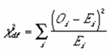
where Oi is the observed frequency and Ei is the expected frequency.
Assumptions – The data are obtained from a random sample. The expected frequency of each category must be at least 5. This goes back to the requirement that the data be normally distributed. You’re simulating a multinomial experiment (using a discrete distribution) with the goodness-of-fit test (and a continuous distribution), and if each expected frequency is at least five then you can use the normal distribution to approximate (much like the binomial).
