A random variable is a variable whose value is determined by the outcome of a random procedure. There are two main types of random variables: discrete and continuous. The modules Discrete probability distributions and Binomial distribution deal with discrete random variables. There is a second type, continuous random variables.
A continuous random variable is one that can take any real value within a specified range. A discrete random variable takes some values and not others; one cannot obtain a value of 4.73 when rolling a fair die. By contrast, a continuous random variable can take any value, in principle, within a specified range.
If a random variable is a continuous variable, its probability distribution is called a continuous probability distribution. A continuous probability distribution differs from a discrete probability distribution in several ways.
- The probability that a continuous random variable will assume a particular value is zero.
- As a result, a continuous probability distribution cannot be expressed in tabular form.
- Instead, an equation or formula is used to describe a continuous probability distribution.
The equation used to describe a continuous probability distribution is called a probability density function (pdf). All probability density functions satisfy the following conditions:
- The random variable Y is a function of X; that is, y = f(x).
- The value of y is greater than or equal to zero for all values of x.
- The total area under the curve of the function is equal to one.
The charts below show two continuous probability distributions. The first chart shows a probability density function described by the equation y = 1 over the range of 0 to 1 and y = 0 elsewhere.
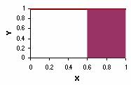
y = 1
The next chart shows a probability density function described by the equation y = 1 – 0.5x over the range of 0 to 2 and y = 0 elsewhere. The area under the curve is equal to 1 for both charts.
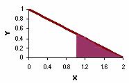
y = 1 – 0.5x
The probability that a continuous random variable falls in the interval between a and b is equal to the area under the pdf curve between a and b. For example, in the first chart above, the shaded area shows the probability that the random variable X will fall between 0.6 and 1.0. That probability is 0.40. And in the second chart, the shaded area shows the probability of falling between 1.0 and 2.0. That probability is 0.25.
Normal Distribution
A distribution is said to be normal when most of the observations are clustered around the mean. It charts a data set of which most of the data points are concentrated around the average (mean) in a symmetrical manner, thus forming a bell-shaped curve. The normal distribution’s shape is unique in that the most frequently occurring value is in the middle of the range and other probabilities tail off symmetrically in both directions. The normal distribution is used for continuous (measurement) data that is symmetric about the mean. The graph of the normal distribution depends on the mean and the variance. When the variance is large, the curve is short and wide and when the variance is small, the curve is tall and narrow.
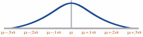
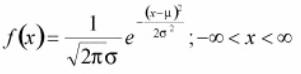
The normal distribution is also called as the Gaussian or standard bell distribution. The population mean μ is zero and that the population variance σ2 equals one as in the figure and σ is the standard deviation. The normal probability density function is
For normal distribution, the area under the curve lies between µ − σ and µ + σ.
Z- transformation – The shape of the normal distribution depends on two factors, the mean and the standard deviation. Every combination of µ and σ represent a unique shape of a normal distribution. Based on the mean and the standard deviation, the complexity involved in the normal distribution can be simplified and it can be converted into the simpler z-distribution. This process leads to the standardized normal distribution, Z = (X − µ)/σ. Because of the complexity of the normal distribution, the standardized normal distribution is often used instead.
Chi-Square Distribution
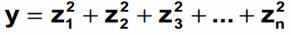
The chi-square (χ2) distribution is used when testing a population variance against a known or assumed value of the population variance. It is skewed to the right or with a long tail toward the large values of the distribution. The overall shape of the distribution will depend on the number of degrees of freedom in a given problem. The degrees of freedom are 1 less than the sample size. It is formed by adding the squares of standard normal random variables. For example, if z is a standard normal random variable, then the following is a chi-square random variable (statistic) with n degrees of freedom
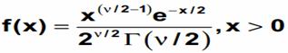
The chi-square probability density function where v is the degree of freedom and (x) is the gamma function is
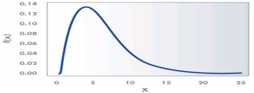
An example of a χ2 distribution with 6 degrees of freedom is as
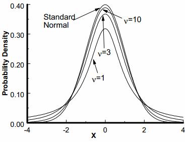
Student t Distribution
It was developed by W.S. Gosset. The t distribution is used to determine the confidence interval of the population mean and confidence statistics when comparing the means of sample populations but, the degrees of freedom for the problem must be know n. The degrees of freedom are 1 less than the sample size.
The student’s t distribution is a symmetrical continuous distribution and similar to the normal distribution, but the extreme tail probabilities are larger than for the normal distribution for sample sizes of less than 31. The shape and area of the t distribution approaches towards the normal distribution as the sample size increases. The t distribution can be used whenever samples are drawn from populations possessing a normal, bell-shaped distribution. There is a family of curves, one for each sample size from n =2 to n = 31.
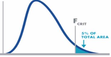
F Distribution
The F distribution or F-test is a tool used for assessing the ratio of independent variances or equality of variances from two normal populations. It is used in the Analysis of Variance (ANOVA, a technique frequently used in the Design of Experiments to test for significant differences in variance within and between test runs).
If U and V are the variances of independent random samples of size n and m taken from normally distributed populations with variances of w and z, then
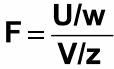
which is a random variable with an F distribution with v1 = n-1 and v2 = m – 1. The F-distribution is represented by

with (s1)2 is the variance of the first sample (n1- 1 degrees of freedom in the numerator) and (s2)2 is the variance of the second sample (n2- 1 degrees of freedom in the denominator), given two random samples drawn from a normal distribution.
The shape of the F distribution is non-symmetrical and will depend on the number of degrees of freedom associated with (s1)2 and (s2)2. The distribution for the ratio of sample variances is skewed to the right (the large values).