A decision tree is a decision support tool that uses a tree-like graph or model of decisions and their possible consequences, including chance event outcomes, resource costs, and utility. It is one way to display an algorithm.
Decision trees are commonly used in operations research, specifically in decision analysis, to help identify a strategy most likely to reach a goal. A decision tree is a flowchart-like structure in which each internal node represents a “test” on an attribute (e.g. whether a coin flip comes up heads or tails), each branch represents the outcome of the test and each leaf node represents a class label (decision taken after computing all attributes). The paths from root to leaf represents classification rules.
In decision analysis a decision tree and the closely related influence diagram are used as a visual and analytical decision support tool, where the expected values (or expected utility) of competing alternatives are calculated.
A decision tree consists of 3 types of nodes:
- Decision nodes – commonly represented by squares
- Chance nodes – represented by circles
- End nodes – represented by triangles
Decision trees are commonly used in operations research and operations management. If in practice decisions have to be taken online with no recall under incomplete knowledge, a decision tree should be paralleled by a probability model as a best choice model or online selection model algorithm. Another use of decision trees is as a descriptive means for calculating conditional probabilities.
Decision trees, influence diagrams, utility functions, and other decision analysis tools and methods are taught to undergraduate students in schools of business, health economics, and public health, and are examples of operations research or management science methods.
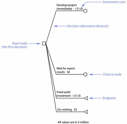
In figure below, a company is evaluating whether to invest $1,000,000 in a project immediately or wait for a marketing report that may affect project development. Two other alternatives are also possible: invest $1,000,000 in a fixed yield bond or do nothing. A fixed-yield investment and doing nothing are examples of baseline alternatives: choices that can be used to compare the overall merits of the decision alternatives.
Elements
Decision nodes and the root node – Small squares identify decision nodes. A decision tree typically begins with a given “first decision.” This first decision is called the root node. For example, the root node in a medical situation might represent a choice to perform an operation immediately, try a chemical treatment, or wait for another opinion. Draw the root node at the left side of the decision tree.
Chance nodes – Small circles identify chance nodes; they represent an event that can result in two or more outcomes. In this illustration two of the decision alternatives connect to chance nodes. Chance nodes may lead to two or more decision or chance nodes.
Endpoints – An endpoint, or termination node, indicates a final outcome for that branch. Small triangles identify endpoints. Show an endpoint by touching one point of the triangle to the branch it terminates.
Branches – Lines that connect nodes are called branches. Branches that emanate from a decision node (and towards the right) are called decision branches. Similarly, branches that emanate from a chance node (and towards the right) are called chance branches. In other words, the node that precedes a branch identifies the branch type. A branch can lead to any of the three node types: decision node, chance node, or endpoint.
Payoff values
The payoff value is equivalent to the net profit (or net loss) expected at the end of any outcome. Write payoff values at their respective branch endpoints. Although you can express payoff in various ways, it is common to use monetary units in most business applications.
Payoff is the difference between investment cost and gross revenue. This primer adopts the convention of indicating investment costs as negative values to simplify calculating payoff values. Payoff values can be positive or negative. Negative payoff values indicate a net loss.
Example
The figure below shows the expected payoffs at two endpoints. The fixed-yield investment results in $1,050,000 revenue, and therefore a $50,000 payoff. The payoff for doing nothing is $0. The other branches lead to chance nodes at this stage of the decision tree. You can assign payoff values only after these chance nodes lead to endpoints.
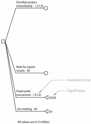
The figure above shows the expected payoffs at two endpoints. The fixed-yield investment results in $1,050,000 revenue, and therefore a $50,000 payoff. The payoff for doing nothing is $0. The other branches lead to chance nodes at this stage of the decision tree. You can assign payoff values only after these chance nodes lead to endpoints.
Outcome probability
A chance node leads to two or more outcomes, each outcome represented by a new branch. As with a game of chance, an outcome has a particular probability of happening. The total of all outcomes for a given chance node must equal 100% (or 1.0). A standard decision tree convention expresses probabilities as decimal fractions in parentheses at the chance branches.
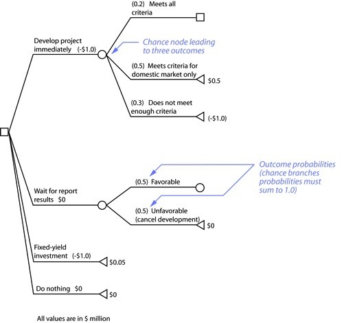
In the figure above, the decision alternative to develop a project immediately can lead to one of three outcomes. The company has determined that there is a 20% chance that the project can meet all the criteria for success in international and domestic markets, but a 50% chance that the project will only meet the criteria for the domestic market. In addition, is a 30% chance that the project will not meet enough criteria for either market as a result of insufficient information.
The company can also wait for a marketing study before developing the project. The marketing information may help the company create a successful project. But the information may also suggest unfavorable conditions that the company probably cannot overcome. The company uses its best judgment and guess, with a 50% favorable and a 50% unfavorable outcome. The decision tree shows these probabilities as decimal fractions in parentheses on their respective chance branches.
Expected Value
Expected value (EV) is a way to measure the relative merits of decision alternatives. The expected value term is a mathematical combination of payoffs and probabilities. You calculate the expected values after all probabilities and payoff values are identified. The goal of the calculations is to find the EV for each decision alternative emerging from the root node. For the purposes of this primer, the decision alternative with the highest EV is the best choice.
Although you can apply the formal definition of expected value, in practice you can calculate EV calculations by applying the following rules. To calculate EV, start from the endpoints and work back towards the root. An easy way to find expected values is to calculate an EV for each terminated branch, then each chance node and each decision node.
For a terminated decision branch, EV is equal to the payoff.
EV = Payoff
For a terminated chance branch, EV is the product of its payoff and probability.
EV = Payoff x Probability
For a chance node, EV is the sum of each chance branch payoff multiplied by the probability for that payoff.
EV = [EV branch1 + EV branch2 + … + EV branchN]
For a decision node, EV is the greatest EV value of all the connected decision branches. Mark the lower value EV branches with double-hatch marks to disregard these branch paths. Since the root node is also the first decision node, the decision alternative with the largest EV is the overall best decision.
EV = the greatest EV value among all the connected decision branches.
The EV at any node becomes the payoff “input” at the node closer to the root.
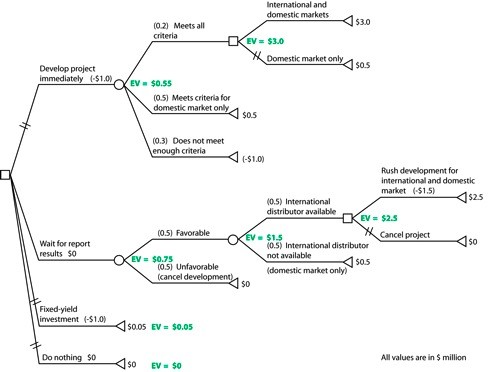
In figure above, calculate the EV for the decision alternative to develop the project by following the given EV rules:
Decision node (“international and domestic marketing” vs. “domestic marketing only”). The EV is the greatest value given by all the decision branches, $3,000,000. This value then becomes the payoff “input” for the next node to the left.
Chance node (“all criteria” vs. “domestic criteria only” vs. “not enough criteria”).
[$3,000,000 x 0.2] + [$500,000 x 0.5] + [(-$1,000,000) x 0.3] = EV = $550,000.This value becomes the payoff “input” for this alternative when considering the root node.
By a similar calculation, the EV for the alternative to wait for the report before deciding whether or not to develop the project is EV = $750,000. This value becomes the payoff “input” for this alternative when considering the root node.
The EV for the alternative to invest the capital in a fixed-yield investment is just the payoff value, EV = $50,000.
The EV for doing nothing is EV = $0.
Decision tree analysis
You analyze a decision tree after all the probabilities, payoff values, and expected values are identified. The decision branch with the highest EV at the root node is the best decision. The results may come as a surprise, so use the decision tree to trace how the results are generated.
You can also see how changing various payoffs or probabilities can affect the results since a decision tree is a system of multiple inputs and outputs. The analyst can change input values to understand how changes affect the system. Use a spreadsheet to alter payoff or probability values to monitor how the analysis changes.
The EV at the root node shows that the decision to wait for the marketing report is the best decision. This result may come as a surprise. Before the decision tree in figure above is analyzed you may be tempted to assume that the decision to develop the project immediately is the better choice. After all, the project will only cost $1,000,000 instead of a rush cost of $1,500,000. Furthermore, there are fewer complications to consider, like waiting to determine the potential for international distribution.
The EV for the decision alternative to wait for the report is complicated by two major chance factors. One factor is that the company knows that waiting makes finding an international distributor more difficult than if the project begins immediately. The company has determined that the likelihood of finding an international distributor is less certain (by 50%) if they wait for the report.
The other chance factor is the information in the marketing report. The company estimates that the marketing report has a 50% chance of delivering favorable data that will help project development. Two or more chance nodes directly connected in this way indicate a dependent uncertainty, a condition that can readily be evaluated through decision tree analysis.
Another complication is that rushing development raises development costs by a third, to (-$1,500,000), and this alone reduces the payoff for the international and domestic marketing by $500,000.
The decision tree method requires probabilities for all chance outcomes. In this example, the successive chance outcomes of waiting for report results and then securing an international distributor reduce the EV along the branch path.
