Linear programming (LP; also called linear optimization) is a method to achieve the best outcome (such as maximum profit or lowest cost) in a mathematical model whose requirements are represented by linear relationships. Linear programming is a special case of mathematical programming (mathematical optimization).
More formally, linear programming is a technique for the optimization of a linear objective function, subject to linear equality and linear inequality constraints.
Optimization models are used extensively in almost all areas of decision-making, such as engineering design and financial portfolio selection. This site presents a focused and structured process for optimization problem formulation, design of optimal strategy, and quality-control tools that include validation, verification, and post-solution activities.
Decision-making problems may be classified into two categories: deterministic and probabilistic decision models. In deterministic models good decisions bring about good outcomes. You get that what you expect; therefore, the outcome is deterministic (i.e., risk-free). This depends largely on how influential the uncontrollable factors are in determining the outcome of a decision, and how much information the decision-maker has in predicting these factors.
Those who manage and control systems of men and equipment face the continuing problem of improving (e.g., optimizing) system performance. The problem may be one of reducing the cost of operation while maintaining an acceptable level of service, and profit of current operations, or providing a higher level of service without increasing cost, maintaining a profitable operation while meeting imposed government regulations, or “improving” one aspect of product quality without reducing quality in another. To identify methods for improvement of system operation, one must construct a synthetic representation or model of the physical system, which could be used to describe the effect of a variety of proposed solutions.
A model is a representation of the reality that captures “the essence” of reality. A photograph is a model of the reality portrayed in the picture. Blood pressure may be used as a model of the health of an individual. A pilot sales campaign may be used to model the response of individuals to a new product. In each case the model captures some aspect of the reality it attempts to represent.
Since a model only captures certain aspects of reality, it may be inappropriate for use in a particular application for it may capture the wrong elements of the reality. Temperature is a model of climatic conditions, but may be inappropriate if one is interested in barometric pressure. A photograph of a person is a model of that individual, but provides little information regarding his or her academic achievement. An equation that predicts annual sales of a particular product is a model of that product, but is of little value if we are interested in the cost of production per unit. Thus, the usefulness of the model is dependent upon the aspect of reality it represents.
If a model does capture the appropriate elements of reality, but capture the elements in a distorted or biased manner, then it still may not be useful. An equation predicting monthly sales volume may be exactly what the sales manager is looking for, but could lead to serious losses if it consistently yields high estimates of sales. A thermometer that reads too high or too low would be of little use in medical diagnosis. A useful model is one that captures the proper elements of reality with acceptable accuracy.
Mathematical optimization is the branch of computational science that seeks to answer the question `What is best?’ for problems in which the quality of any answer can be expressed as a numerical value. Such problems arise in all areas of business, physical, chemical and biological sciences, engineering, architecture, economics, and management. The range of techniques available to solve them is nearly as wide.
A mathematical optimization model consists of an objective function and a set of constraints expressed in the form of a system of equations or inequalities. Optimization models are used extensively in almost all areas of decision-making such as engineering design, and financial portfolio selection. This site presents a focused and structured process for optimization analysis, design of optimal strategy, and controlled process that includes validation, verification, and post-solution activities.
If the mathematical model is a valid representation of the performance of the system, as shown by applying the appropriate analytical techniques, then the solution obtained from the model should also be the solution to the system problem. The effectiveness of the results of the application of any optimization technique, is largely a function of the degree to which the model represents the system studied.
To define those conditions that will lead to the solution of a systems problem, the analyst must first identify a criterion by which the performance of the system may be measured. This criterion is often referred to as the measure of the system performance or the measure of effectiveness. In business applications, the measure of effectiveness is often either cost or profit, while government applications more often in terms of a benefit-to-cost ratio.
Optimization-Modeling Process
Optimization problems are ubiquitous in the mathematical modeling of real world systems and cover a very broad range of applications. These applications arise in all branches of Economics, Finance, Chemistry, Materials Science, Astronomy, Physics, Structural and Molecular Biology, Engineering, Computer Science, and Medicine.
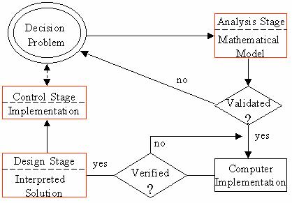
Optimization modeling requires appropriate time. The general procedure that can be used in the process cycle of modeling is to: (1) describe the problem, (2) prescribe a solution, and (3) control the problem by assessing/updating the optimal solution continuously, while changing the parameters and structure of the problem. Clearly, there are always feedback loops among these general steps.
- Mathematical Formulation of the Problem: As soon as you detect a problem, think about and understand it in order to adequately describe the problem in writing. Develop a mathematical model or framework to re-present reality in order to devise/use an optimization solution algorithm. The problem formulation must be validated before it is offered a solution. A good mathematical formulation for optimization must be both inclusive (i.e., it includes what belongs to the problem) and exclusive (i.e., shaved-off what does not belong to the problem).
- Find an Optimal Solution: This is an identification of a solution algorithm and its implementation stage. The only good plan is an implemented plan, which stays implemented!
- Managerial Interpretations of the Optimal Solution: Once you recognize the algorithm and determine the appropriate module of software to apply, utilize software to obtain the optimal strategy. Next, the solution will be presented to the decision-maker in the same style and language used by the decision-maker. This means providing managerial interpretations of the strategic solution in layman’s terms, not just handing the decision-maker a computer printout.
- Post-Solution Analysis: These activities include updating the optimal solution in order to control the problem. In this ever-changing world, it is crucial to periodically update the optimal solution to any given optimization problem. A model that was valid may lose validity due to changing conditions, thus becoming an inaccurate representation of reality and adversely affecting the ability of the decision-maker to make good decisions. The optimization model you create should be able to cope with changes.
- The Importance of Feedback and Control: It is necessary to place heavy emphasis on the importance of thinking about the feedback and control aspects of an optimization problem. It would be a mistake to discuss the context of the optimization-modeling process and ignore the fact that one can never expect to find a never-changing, immutable solution to a decision problem. The very nature of the optimal strategy’s environment is changing, and therefore feedback and control are an important part of the optimization-modeling process.
The above process is depicted as the Systems Analysis, Design, and Control stages in the following flow chart, including the validation and verification activities:
Linear Programming
Linear programming (LP) is a powerful framework for describing and solving optimization problems. It allows you to specify a set of decision variables, and a linear objective and a set of linear constraints on these variables. To give a simple and widely used example, consider the problem of minimizing the cost of a selection of foods that meets all the recommended daily nutrient guidelines. The LP model would have a set of decision variables that capture the amount of each food to buy, a linear objective that minimizes the total cost of purchasing the chosen foods, and a linear constraint for each nutrient, requiring that the chosen foods together contain a sufficient quantity of that nutrient.
Using linear algebra notation, a linear program can be described as follows:
Objective: minimize cTx
Constraints: A x = b (linear constraints)
l ≤ x ≤ u (bound constraints)
When described in this form, the vector x represents the decision variables, the vector c captures the linear objective function, the matrix equation Ax = b specifies the linear constraints on x, and the vectors l and u give the lower and upper bounds on x.
A linear programming problem is said to be in “standard form” when it is written as:
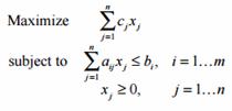
The problem has m variables and n constraints. It may be written using vector terminology as:
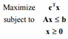
A problem where we would like to minimize the cost function instead of maximize it may be rewritten in standard form by negating the cost coefficients cj (c )T.
Any vector x satisfying the constraints of the linear programming problem is called a feasible solution of the problem. Every linear programming problem falls into one of three categories:
- A linear programming problem is infeasible if a feasible solution to the problem does not exist; that is, there is no vector x for which all the constraints of the problem are satisfied.
- A linear programming problem is unbounded if the constraints do not sufficiently restrain the cost function so that for any given feasible solution, another feasible solution can be found that makes a further improvement to the cost function.
- Has an optimal solution. Linear programming problems that are not infeasible or unbounded have an optimal solution; that is, the cost function has a unique minimum (or maximum) cost function value. This does not mean that the values of the variables that yield that optimal solution are unique, however.
The basic algorithm most often used to solve linear programming problems is called the simplex method. Over the past 50 years, it has been developed to the point that good computer programs using the simplex method and its relatives (the revised simplex method and the network simplex method) can solve virtually any bounded, feasible linear programming problem of reasonable size in a reasonable amount of time. Only in the past ten years have other methods of solving linear programming problems (so-called interior point methods) developed to the point where they can be used to solve practical problems.
The Simplex Method
The simplex method has two basic steps, often called “phases.” The first phase is to find a feasible solution to the problem. For small problems, or larger problems of certain forms, this is not at all difficult. Often, a trivial solution such as x = 0 is a feasible solution, as in the production planning problem described earlier. We will omit the details of solving the first phase to find a feasible solution for now.
After a feasible solution to the problem is found, the simplex method works by iteratively improving the value of the cost function. This is accomplished by finding a variable in the problem that can be increased, at the expense of decreasing another variable, in such a way as to effect an overall improvement in the cost function. This can be visualized graphically as moving along the edges of a feasible set from corner to corner.
Consider the linear programming problem:
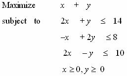
The feasible set of this problem can be graphed in two dimensions as shown in the following figure. The non-zero constraints x 0 and y 0 confine the feasible set to the first quadrant. The other three constraints are lines in the x-y plane, as shown. The cost function, x + y, can be represented as a line of slope –1 with any intercept. The value of the intercept of the cost function line is the value of the cost function for any solution that lies along that line. The heavy line in the following represents the optimal solution of the problem, since it is the line with slope –1 with the maximum intercept (10) that intersects the feasible set. The value of the cost function for this optimal solution is 10, and the cost function line x + y = 10 has exactly one point in the feasible set, x = 4, y = 6.
The simplex method works by finding a feasible solution, and then moving from that point to any vertex of the feasible set that improves the cost function. Eventually a corner is reached from which any movement does not improve the cost function. This is the optimal solution. In this example, x = 0 and y = 0 is a trivial feasible solution, and has a cost function value of 0. This is vertex A in the figure. From this point, we can either move to point B or point E. Point E (0, 4) increases the cost function to 4, while point B (5, 0) increases it to 5. Since point B gives us more improvement, we will select it as our first iteration. The value of x increases from 0 to 5, while y remains 0.
From point B, it is necessary to check whether a move to point C is advantageous. (We know that moving back to A is not.) Point C (6, 2) has a cost function value of 8, which is an improvement. Therefore we increase x from 5 to 6, which means that because of the constraints 2x – y < 10 and –x + 2y > 8, we must also increase y from 0 to 2. From point C, we now check whether a move to point D improves the situation. The cost function at D (4, 6) is 10, so the move is accepted and increased y from 2 to 6. This means that x must decrease from 6 to 4 because of the constraints. Now, since a move to either point E (cost function value of 4) or point C (cost function value of 8) decreases the cost function, it is known that point D is the optimal solution to this problem.
When you formulate a decision-making problem as a linear program, you must check the following conditions:
- The objective function must be linear. That is, check if all variables have power of 1 and they are added or subtracted (not divided or multiplied)
- The objective must be either maximization or minimization of a linear function. The objective must represent the goal of the decision-maker
- The constraints must also be linear. Moreover, the constraint must be of the following forms ( <, >, or =, that is, the LP-constraints are always closed).
Any linear program consists of four parts: a set of decision variables, the parameters, the objective function, and a set of constraints. In formulating a given decision problem in mathematical form, you should practice understanding the problem (i.e., formulating a mental model) by carefully reading and re-reading the problem statement. While trying to understand the problem, ask yourself the following general questions:
- What are the decision variables? That is, what are controllable inputs? Define the decision variables precisely, using descriptive names. Remember that the controllable inputs are also known as controllable activities, decision variables, and decision activities.
- What are the parameters? That is, what are the uncontrollable inputs? These are usually the given constant numerical values. Define the parameters precisely, using descriptive names.
- What is the objective? What is the objective function? Also, what does the owner of the problem want? How the objective is related to his decision variables? Is it a maximization or minimization problem? The objective represents the goal of the decision-maker.
- What are the constraints? That is, what requirements must be met? Should I use inequality or equality type of constraint? What are the connections among variables? Write them out in words before putting them in mathematical form.
Example
You need to buy some filing cabinets. You know that Cabinet X costs $10 per unit, requires six square feet of floor space, and holds eight cubic feet of files. Cabinet Y costs $20 per unit, requires eight square feet of floor space, and holds twelve cubic feet of files. You have been given $140 for this purchase, though you don’t have to spend that much. The office has room for no more than 72 square feet of cabinets. How many of which model should you buy, in order to maximize storage volume?
The question ask for the number of cabinets I need to buy, so my variables will stand for that:
x: number of model X cabinets purchased
y: number of model Y cabinets purchased
Naturally, x > 0 and y > 0. I have to consider costs and floor space (the “footprint” of each unit), while maximizing the storage volume, so costs and floor space will be my constraints, while volume will be my optimization equation.
cost: 10x + 20y < 140, or y < –( 1/2 )x + 7
space: 6x + 8y < 72, or y < –( 3/4 )x + 9
volume: V = 8x + 12y
This system (along with the first two constraints) graphs as:
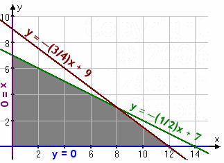
When you test the corner points at (8, 3), (0, 7), and (12, 0), you should obtain a maximal volume of 100 cubic feet by buying eight of model X and three of model Y.
