After having described the sampling process, let us discuss the types of sample designs. Of the designs covered here, quota sampling, judgment sampling and convenience sampling are the non-probability sample designs; the remaining ones are probability sample designs.
Random Sampling: A random sample gives every unit of the population a known and non-zero probability of being selected. Since random sampling implies equal probability to every unit in the population, it is necessary that the selection of the sample must be free from human judgment.
There is some confusion between the two terms ‘random sampling’ and ‘unrestricted random sampling’. In the latter case, each unit in the population has an equal chance of being selected in the sample. Such a sample is drawn ‘with replacement’, which means that the unit selected at each draw is replaced into the population before another draw is made from it. As such, a unit can be included more than once in the sample. Most statistical theory relates to ‘unrestricted random sampling’. In order to distinguish between these two samples, i.e. sample, without replacement and sample with replacement, the terms ‘simple random sample’ and ‘unrestricted random sample’ are used. If the latter is devised in such a manner that no unit can be included more than once, it will then be known as the simple random sampling.
It may be noted that while both simple random sampling and unrestricted random sampling give an equal probability to each unit of the population for being included in the sample, there are other sample designs too which provide equal probability to the units. The process of randomness is the very core of simple and unrestricted random sampling. The selection of a sample must be free from bias which can be ensured only when the process of selection is free from human judgment.
As Moser and Kaltonhave observed, “the definition of randomness relates to the mode of selection, not to the resultant sample”. The significance of this statement must be clearly understood.
Despite the method of random selection used for drawing a sample, the outcome may not be a representative sample. Since the means of sample distribution constitute a normal distribution, a sample selected may be “close to one of the tails of the sampling distribution”. Though the probability of such a situation would be rather remote, it does exist. One cannot doubt the process of randomness on the basis of the unrepresentative nature of a single sample. Once in a while, an unrepresentative sample may be obtained through the random process. In such a case, another sample could be drawn so that it is really representative. However, if on repeated draws one finds that the samples are not representative, then one can question the validity of random selection itself.
The process of randomness does not mean that it is ‘haphazard’, as a layman may be inclined to think. What it means is that the process of selecting a single is independent of human judgment. To ensure this, there are two methods that are followed when drawing a random sample. These are:
(i) The lottery method and (ii) the use of random numbers. In the lottery method, each unit of the population is numbered and shown on a chit of paper or disc. The chits are folded and put in a box from which a sample of the requisite size is to be drawn. In case discs are used, there are well mixed up before a draw is made so that no particular unit can be identified before it gets selected. In the second method, the tables of random numbers are used. The members of the population are numbered from 1 to N from which n members are selected. This process is explained below with the help of an illustration.
Suppose a sample of size 50 is to be selected from a population of 500. First, number the 500 units from 1 to 500, the order being quite immaterial. While numbering the units, ensure that each unit in the population has uniform digits, in this case, three. Thus, 1st unit would have a three digit number 001, 2nd unit 002, 10th unit 010, 11th unit 011, and so on. After the units have been given three-digit numbers, the table of random numbers is to be used. One may start from the left-hand top corner of the table of random numbers and proceed systematically down sets of three-digit columns, rejecting numbers over 500 and those which have occurred earlier.
Using the first thousand numbers from the table of random numbers, a sample of 50 out of 500 will thus be chosen.
Sample of 50
| 231 | 092 | 434 | 318 | 032 |
| 055 | 259 | 325 | 263 | 194 |
| 148 | 113 | 211 | 239 | 144 |
| 389 | 455 | 207 | 108 | 337 |
| 117 | 126 | 398 | 379 | 224 |
| 433 | 426 | 225 | 420 | 006 |
| 495 | 062 | 485 | 122 | 068 |
| 367 | 401 | 035 | 441 | 043 |
| 070 | 100 | 171 | 493 | 500 |
| 313 | 488 | 047 | 310 | 222 |
Systematic Sampling: In practice, the method followed in systematic sampling is simpler than that explained earlier. First, a sampling fraction is calculated. For instance, in the foregoing example, a sample of 50 out of 500 units was chosen. The sampling fraction k is N/n where N is the total number of units in the population and n is the size of the sample. In the above example, k is 500/50 = 10. Second, a number between 1 and 10 is chosen at random. Suppose the number thus selected happens to be 9. Then, the sample will comprise numbers 9, 19, 29, 39, 49, 489 and 499.
If will be seen that it is extremely convenient to select a sample in this way. The main point to note is that once the first unit in the sample is selected, the selection of subsequent units in the sample becomes obvious. In view of this, it has been questioned whether the process of selection for subsequent units is random. Here, the selection of a unit is dependent on the selection of a preceding unit in contrast to simple random sampling where the selection of units is independent of each other. Systematic random sampling is sometimes called quasi-random sampling.
Stratified Random Sampling: A stratified random sample is one where the population is divided into mutually exclusive and mutually exhaustive strata or sub-groups and then a simple random sample is selected within each of the strata or sub-groups. Thus, human population may be divided into different strata on the basis of sex, age groups, occupation, education or regions. It may be noted that stratification does not mean absence of randomness. All that it means is that the population is first divided into certain strata and then a simple random sample is chosen within each stratum of the population.
The following example will make this clear:
| Strata income per month (Rs) | Population Number of Households | Sample(Proportionate) | Sample (Disproportionate) |
| 0-500 | 5,000 | 50 | 75 |
| 501-1000 | 4,000 | 40 | 20 |
| 1001-2000 | 3,000 | 30 | 20 |
| 2001-3000 | 2,000 | 20 | 25 |
| 3001+ | 1,000 | 10 | 10 |
| ________ | ________ | __________ | |
| 15,000 | 150 | 150 |
In the above example, the population consists of 15,000 households, divided into five strata on the basis of monthly income. Column (3) of the table shows the sample, i.e., number of households selected from each stratum. The sample constitutes one per cent of the population. A sample of this type, where each stratum has a uniform sampling fraction, is called a proportionate stratified sample. If, on the contrary, the strata have variable sampling fractions, the sample is called a disproportionate stratified sample. The figures given in column (4) of the above table show a disproportionate stratified sample. It will be seen that the sampling fraction varies from the stratum to another. Thus, for example, it is 0.015 for the monthly income Rs.0-500 and 0.01 for the stratum, Rs.3001 +.
It may be noted that a stratified random sample with a uniform sample fraction results in greater precision than a simple random sample. But, this is possible only when the selection within strata is made on a random basis. Further, a stratified proportionate sample is generally convenient on account of practical considerations.
There are some other considerations in favour of the stratified random sample. The researcher may be interested in the results for separate strata rather than for the entire population. A simple random sample will not show results by strata as it presents only an aggregative picture. Another consideration is that it may be administratively expedient to split the population into strata. Thus, the population of a country may be divided into regions, states or districts, so that each of these strata may be put under the charge of a separate supervisor. Yet another consideration could be that one can use different procedures for selecting samples from various strata. Thus, the procedure to select sample households in rural areas may be altogether different from that followed in urban areas. If the data are more variable in strata, a larger sampling fraction in those strata should be taken. This would result in greater overall precision.
Estimation of the Universe Mean, With A Stratified Random Sample
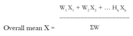
In the preceding pages, we have seen that a stratified random sample comprises a group of simple random samples drawn from strata into which the population has been classified. The simple mean of each stratum is unbiased. To obtain an unbiased estimate of the population mean, the means of the individual strata should be combined. This is possible by taking a weighted mean of the individual strata means. A numerical example will make this point clear.
Suppose there are three strata in a population. A stratified random sample covering 10 observations, in all, was selected, with the following particulars:
| Stratum Number | Number of Observations | Value of each observation | Total value of all observations |
| 1 | 3 | 5,10,15 | 30 |
| 2 | 5 | 20,25,15,30,10 | 100 |
| 3 | 2 | 35,25 | 60 |
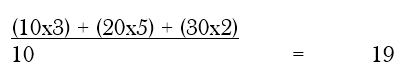
In order to calculate the sample mean for each stratum, the total value of all observations is to be divided by the number of observations. Thus, the sample means are 10, 20 and 30 for stratum 1, 2 and 3 respectively. These means are to be combined into an overall mean. For this purpose, weights are to be assigned to each stratum on the basis of the proportion of the number of observations in the stratum to the total number of observations in the population. Thus, a weight of 3, 5 and 2 should be assigned to the three strata, in that order. Now, the overall mean of the sample mean in the three strata can be calculated as follows:
Let us take another example. Suppose we have the following data on consumption of sample households
| Income Stratum | Sample mean purchase per household | Number of households In stratum |
| Rich | 3,000 | 10,000 |
| Middle class | 1,200 | 30,000 |
| Poor | 500 | 60,000 |
Then the estimated population mean monthly expenditure per household would be:
XSY
= W1 X1 + W2 X2 + W3 X3
= (0.1) (3000) + (0.3) (1200) + (0.6) (500)
= 300 + 360 + 300
= Rs.960
Now, we may generate this, symbolically, as follows:
| Stratum | Sample mean in stratum | Sample mean in stratum |
| 1 | X1 | W1 |
| 2 | X2 | W2 |
| . | . | . |
| . | . | . |
| . | . | . |
| h | Xh | Wh |
Estimation of confidence interval with stratified random sample Having calculated the population mean from the sample means for different strata, it is now necessary to estimate its confidence interval. First, an estimate of standard error is to be obtained on the same lines as in the simple random sampling. Second, the estimated standard error is to be multiplied by an appropriate figure (say, by two for 95 per cent confidence and by three for almost 100 per cent confidence), depending upon the degree of confidence desired. Finally, the figure obtained in the preceding step is added to a subtracted from the estimated population mean. This will result in two numbers which are the confidence limits.
In order to estimate the standard error of the mean, it is necessary to have data on sample variance, sample size, and weight for each stratum. Symbolically, the data requirement can be shown as follows:
| Stratum | Sample variance in stratum | Sample size in stratum | Weight of Stratum |
| 1 | S12 | N1 | W1 |
| 2 | S22 | N2 | W2 |
| . | . | . | |
| . | . | . | |
| . | . | . | |
| B | Sb2 | Nh | Wh |
where S1 2 is the variance of the sample in stratum 1, n1 is the number of observations or items in stratum 1, and W1 is the weight of stratum 1, indicating its relative importance. In the same manner, for stratum 2, the sample variance is S2 2, the sample size is n2 and the weight W2. The subscripts 1, 2 ……h indicate the number of strata.
For estimating the standard error, the following formula may be used:
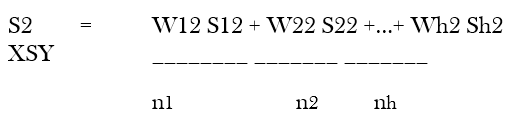
This gives the value of S2 XSY the square root of which is the standard error.
As in illustration, suppose we have the following data pertaining to consumption of sample households in three strata – rich, middle-class and poor.
| Income Stratum | Sample variance in stratum (S2) | Sample size in stratum (n) | Weight of Stratum (W) |
| Rich | 6,000 | 60 | 0.1 |
| Middle class | 4,000 | 100 | 0.3 |
| Poor | 1,200 | 240 | 0.6 |
The required calculations will be as follows:
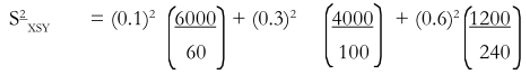
= (0.01 x 100) x (0.09 x 40) x (0.36 x 5)
= 1 + 3.60 + 1.80
= 6.4
The standard error of the mean is
As 95 per cent confidence interval is between ± 2 standard error, it is necessary to multiply the standard error by 2. This gives a figure of 5.06. This should be added to and subtracted from the sample mean of Rs.960 (previous example). This gives a 95 per cent confidence interval of Rs.954.94 to 965.06. If we take ± 3 as the standard error, then we can get an interval which is almost certain to cover the population mean
Rs.960 ± 3 (5.06)
or Rs.960 – 15.18 and
Rs.960 + 15.18
or Rs.944.82 to Rs.975.18
It may be noted that in the above calculations, differences among strata means did not enter into the standard error, unlike the simple random sample. The calculations were based on the estimated within-stratum variances. It is because of this reason that a stratified random sampling gives a more precise estimate of the population mean than a simple random sampling for a given sample size.
There are three major issues in stratified sampling:
- Bases of stratification
- Number of strata
- Sample sizes within strata
