Various types of quantitative models (or operations research models) have been used to help determine the best facilities location. Let us describe a few models that are simple to understand and powerful enough to give some good answers that could aid you in taking a location decision.
Median Model
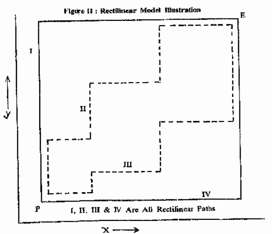
Let us discuss the simple median model which is based on the assumption that the mode of interaction or the path of movement/transportation of load is done on a rectangular/rectilinear pattern. The movement is similar to the movement of `rooks’ on a chess board. Thus all movements are made horizontally along and east-west and/or vertically in a north-south direction. Diagonal moves are not considered. You could refer to Figure II for a diagrammatic portrayal of the rectilinear path. The paths I, II, III and IV are all alternative rectilinear paths between two reference points say a new facility, P, having coordinate locations (x, y) and an ancillary existing facility, A having coordinate locations (a;, b;). Though there are alternative rectilinear paths, the rectilinear distance between the points A and P is however unique and it is mathematically stated as
Dr = Rectilinear Distance = x-ai + y-bi
Now there would be some interaction by way of say the annual number of loads to be moved between two reference points. We could safely assume that the transportation cost for a load is proportional to the distance for which it is moved. This assumption could be questioned on the plea that there is a `telescopic’ scheme of rates charged in actual practice by Indian Railways. The total transportation cost is obtained by adding the number of loads to the times the rectilinear distance is moved.
(TC) Total Transportation Cost = ∑Li × Di i=1
Where L; is the number of loads to be moved between the new facility to be located and the ancillary existing Ph facility (say raw material sources or market distribution outlet points), D; is the rectilinear distance between a new facility and ith existing facility and `m’ is the number of ancillary existing facilities.
Thus as a Location analyst, we essentially want to determine the `least transportation cost’ location solution. The simple median model can help answer this question by using these three steps.
- Identify the median value of the total number of loads moved.
- Find the X-coordinate value of the existing facility that sends (or receives) the median load and
- Find the Y-coordinate value of the existing facility that sends (or receives) the median load.
The x and y values found in steps (ii) and (iii) define the desired optimal (best) location of the new facility.
Let us illustrate the above steps with a small example. Let us assume that a new processing plant is to be located. It would be receiving certain raw materials from two supply sources, S t and S2. It would be sending its finished products to two distribution points, Dl and D2. The coordinate locations of the sources and distribution points are shown in Figure III below.
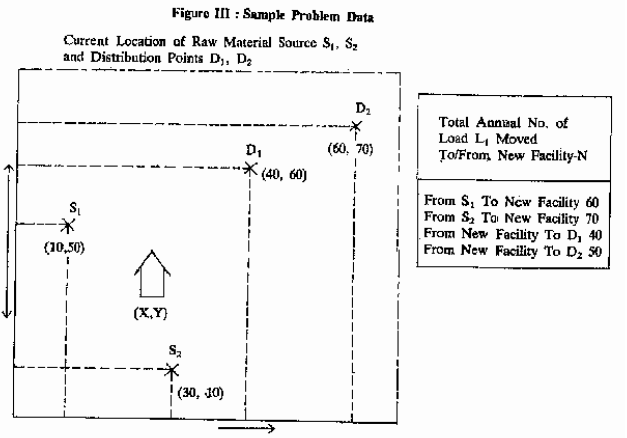
Now in step (i), we have to identify the median value of the total number of loads moved. The total load moved is 220 (viz. 60+70+40+50=220). The median number of loads is the value that has half an equal number of loads above and below it. When the total number of loads is odd, the median load is the middle load; in case of an even number, the median loads are the two, middle loads. Thus for 220 loads, the median loads are 111 and 110 since there are 109 above and below this pair of values.
In step (ii) Let us now determine the X-coordinate of the median load. We could place in an ascending order the x-co-ordinates of the existing facilities viz. it is just going horizontally from left to right in Figure II. Thus the order of the existing facilities would be as S t , S2, D t and. D 2 having annual loads of movement of 60,70, 40 and 50, respectively. Loads 1 to 60 ‘are shipped by source St at X = 10, Loads 61 to 130 are shipped by source S 2 at X 2 =30. Since the median loads (110) and (Ill) fall in the interval 61 to 130, therefore, x=30 is the best x-co-ordinate location for the new facility.
Similarly, in step (iii), we can determine the y-co-ordinate of the median load. In this case we move vertically upwards. From Figure; Ill, it can readily be seen that this ascending order would be represented by the existing facilities S2, S i, D 1and D 2 with annual movement of loads to the tune of! 70, 60, 40 and 50, respectively Loads 1 to 70 are shipped by source S 2 at Y 2 =10. Loads 71 to 130 are shipped by source S i at Yi =50. Since the median loads (110 and Ill) fall in the interval 71 to 130, therefore Y=50 is the best Y-coordinate location for the new facility.
Thus the optimal best location for the new manufacturing facility is (x = 30, Y = 50). Facilities Location at this point minimizes annual transportation costs for the above production distribution system.
TC = ∑Li. Di
Now the total transportation cost as explained earlier on is i=1 and as
Di is the rectilinear distance
TC = ∑[Li¦x-ai¦+¦y-bi¦] i=1
Let us assume that each distance unit cost is Re. 1 per load.
At x = 30, y = 50 viz. the optimal location of the new facility, the total cost TC can be computed as follows:
- Cost for S, to New Facility = 60 [130 -10 I+ 150- 501] = 60 (20+ 10) = 1200
- Cost for S2 to New Facility = 70 [130- 30 I+ 150-101] = 70 (0 + 40)=2800
- Cost for New Facility to D, 40 [130 – 40 I+ 150 – 601 ] = 40 (10+10) = 800
- Cost from New Facility to D2 = 50 [130 – 60 I + 150 -701] = 50 (30 + 20) = 2500
TC = (a) + (b) + (c) + (d) = 1,200 + 2, 800 + 800 + 2,500
viz. TC = 7,300
Activity C
Supposing the new facility is located at a place at x = 50, y = 30. What would be the total transportation costs in this case? Is it a better location than the new location at a (x = 30, y 50)?
- The median model is very simple to operate. It could suffer from some major disadvantages such as:
- It assumes that only one single new facility is to be located
- Every point in the (x, y) plane has been assumed to be an eligible point for the location of the new facility.
- The median model is valid when the movement is based on a rectilinear mode only.
Let us now look .at another model, which though a single facility model, doesn’t assume the rectilinear mode of interaction. This is popularly known as the Gravity Model.
The Gravity Model
The technique determines the low cost `Centre of Gravity’ location of a new facility with respect to the fixed ancillary existing facilities like source suppliers (S1,S2 etc.) and distribution points (D1,D2 etc.) for which each type of product consumed or sold is known. Let us use the same data as that of the median model and thus let us refer to Figure III once more. The only difference is the mode of interaction between the single new facility and the existing facilities. In this case we assume that all goods move in a straight line joining the ancillary facility and the new facility. This is the so-called Euclidean’ mode of interaction and is in fact the shortest distance between any two reference points.
Thus De =Euclidean Distance = [(x-ai)2+(y-bi)] 1/2
Thus the total transportation costs in this case are m
∑(LiDi)
TCe (Total transportation cost) (Euclidean case) = i=1
∑
viz TCe= i=1 Li [/x-ai / 2+ / y-bj / 2]
Our aim, once again, is to determine the location of the new facility at (x,y) such that TCe ,viz. the total transportation costs are as minimum. We will not get into a discussion on certain analytical problems and difficulties in obtaining optimal solutions at this stage/level, but rather present an analogue model and a gravity model which are simple to understand and could be readily applied.
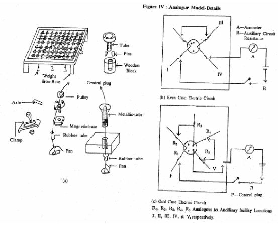
The concept underlying the technique is best visualized as a series of strings to which are attached weights corresponding to the loads/weights of raw materials consumed/dispatched at each source and of finished goods sold/received at each distribution point/market. The strings are threaded through holes in a flat plain metallic sheet; the holes correspond to the ancillary facility locations. The other ends of the string are tied together to a small concentric ring. The ring will finally reach an equilibrium based on the principle of equilibrium of coplanar forces. This equilibrium will be the centre of mass or the ton-mile centre. It is for this reason that this model is also called the Gravity Model. This mechanical analogue model constructed on a Varignon frame does suffer on account of friction. Banwet2 and Vrat have devised a superior. Electro-mechanical analogue model, the details of which are given in Figure IV The electrical analogue depends on making an appropriate electrical series circuit. The resistivity of the wire in resistance per unit length is synonymous to the weights/loads. Due care and precautions have to be taken for preventing short circuits by appropriate insulation devices. It will be noticed that when the central plug/ring is moved to different locations, the total resistance in the circuit changes. Determining a point with minimum total resistance is analogous to the gravity solution viz. the least cost location solution.
x = ∑Li (ai ) i=1 y = ∑Li (bi ) i=1
∑ i i=1 ∑ i i=1
Thus for our example under discussion now from supply sources S1, S2 to the new facility
∑L =60+70 =130 i=1
∑(Lai ) =(60×10)+(70×30) =600+2100 = 2700 i=1
and from new facility to distribution points D; and D2
∑(L ) = 40+50 =90 i=1
∑(Lai ) =(40×40)+(50×60) =1,600+3,000 = 4,600 i=1
∑Liai (source-new facility)+∑Liai (New facility – distribution points) X= i=1 i=1
∑Li (source-new facility) +∑Li (New facility – distribution points) i=1 i=1
X = 2700+4600 = 7300 =33.19
130+90 220
Similarly y can be determined on similar lines from supply sources to the new facility,
∑(Lb ) =(60×50)+(70×10) =3000+700 =3700 i=1
and from the new facility to the distribution points
∑(Lb ) =(40×60)+(50×70) = 2400+3500 =5900 i=1
∑Li = 220
Total load i=1 as before
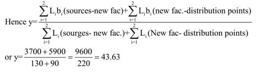
Thus the gravity model solution is to locate the new facility at a point (33.19, 43.63) for which least total transportation costs would be incurred in the case of Euclidean (strictly square of Euclidean) mode of interaction.
Let us compare the results of the median and gravity models. The median model for the rectilinear mode of interaction assumption gives the optimal location of the facility at (30, 50) whereas the gravity model for the Euclidean (strictly squared Euclidean) mode of interaction gives the optimal location of (33.10,43.63). It is therefore necessary for the modeler to know the exact nature of the mode of interaction between the new and ancillary facilities; it is quite possible that the location solution could be highly sensitive to the mode of interaction.
You would have noticed that we have only discussed the location problems dealing with just a single new facility and also what is termed as a minisium objective of minimizing the sum of weighted appropriate distances. There could be cases when the location as determined above turns out to be non-feasible, because of existence of certain restrictions or limitations. Methods are available for drawing iso-cost contour lines which aid the decision maker to take subsequent appropriate decisions. Sometimes a minima objective might be more suited in which case the location analyst attempts to minimize the maximum weighted appropriate distances. Such a criterion would be applicable in emergency like facility location problems of fire stations, hospitals etc. Magnesium objective situations are appropriate for locating factories, warehouses etc.
There are quite a few operational research techniques that aid the location analyst. Some of these are linear programming, transportation along with, heuristic programming, simulation, direct search procedures, graph theory, goal programming etc. Ban wet has given a comprehensive review and progress in facilities location which could be referred to by those interested in further reading on the subject.
You would have observed that facilities location decision is based on a set of factors some of which are tangible/objective whereas some are intangible/ subjective in nature. Brown and Gibson have proposed a composite location measure to aid the decision makers.
Composite Location Measure Model-2
Let us now discuss Brown Gibsons model which provides a composite location measure of the objective and subjective factors. We illustrate the procedure with the help of an example,
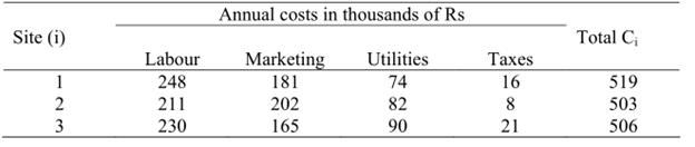
Step-1 First of all identify the factors that deserve to be included in the study and determine which of these must be absolutely satisfied, e.g., there is no point in choosing a site having a scarcity of water whereas the plant requires an abundant water supply. Say the objective factors are labour, marketing, utilities and taxes. Now for the subjective factors, these could include housing, recreation and competition.
Step-2 Let us derive an objective factor (OF) for it location site by multiplying that
∑(1/Ci ),
site’s rupee cost (Ci) by the sum of the reciprocals of all the costs and take the inverse of the product.
OF=[c1 ×∑(1/ci )] -1
Viz
Thus if we have the following data for three possible sites, OF can be obtained as below:
Annual costs in thousands of Rs
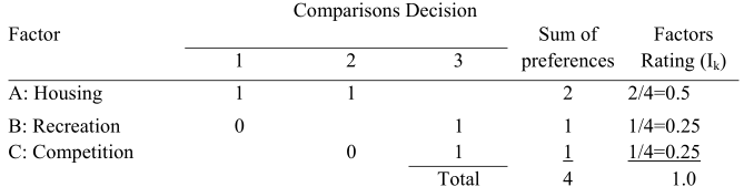
Step-3. Let us now deal with the subjective intangible factors with the help of a forced pair-wise comparison rating method. This procedure is first applied to rank the importance of the factors (Ik) for housing, recreation and competition; and is then applied to each site to rate how well that site satisfies the factors (Sik). These two ratings are combined to obtain a subjective factor (SFi) ranking for each site as
SFi = ∑(Ik . Sik )
The factor comparison is made in pairs. If one factor is preferred over the other, the one preferred is given 1. point whereas the other factor is given 0 points. Thus the table below is quite self-explanatory. If one is indifferent between the two factors, 1 point each can be assigned as seen in decision 3 while comparing factors B and C. 54
Next each of its factors A, B and C is then evaluated for site preferences in a similar manner
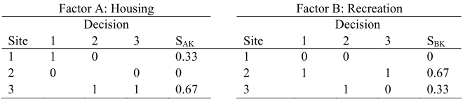
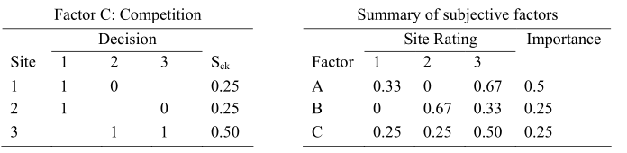
We can now calculate the subjective factor value (SFi) for each site as follows:
SF1 = (0.5) (0.33) + (0.25) (0) + (0.25) (0.25) = 0.2275
SF2 = (0.5) (0) + (0.25) (0.67) + (0.25) (0.25) = 0.2300
SF3 = (0.5) (0.67) + (0.25) (0.33) + (0.25) (0.50) = 0.5425
Step-4: Now depending on the parties concerned would depend a weight age (X) given to the objective versus subjective factors. Let us say we give a two thirds weight age to objective and only one third weight age to the subjective factors.
Viz, X = 0.667.
Step-5: Assuming that all sites that failed to meet the minimum levels set for the critical factors in step-1 have been eliminated for the remaining sites, a composite location measure (LMi) can be obtained as follows:
(LMi) = X (OF) + (1-X) SFi
Using the data generated in steps 2, 3 and 4, we have
LMi = 0.67 (0.3271) + 0.33 (0.2275) = 0.2942
LM2 0.67 (0.3375) + 0.33 (0.2300) = 0.3020
LM3 = 0.67 (0.3355) + 0.33 (0.5425) = 0.4038
The site 3 is preferred. A sensitivity analysis could be done by varying the values of X. It will be seen that if X is very close to 1, site 2 would be preferred.
Bridgeman’s Dimensional Analysis
As has already been observed, while selecting plant locations, we want to optimize different objectives which are interrelated but cannot be represented in the same dimensions. The location decision can be taken by making use of Bridgeman’s dimensional analysis. Let us construct the utility payoff matrix once again as shown in Table below:
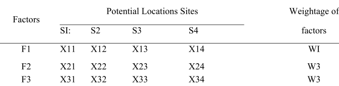
where Xij = utility of having the plant in” location j with respect to the ith factor. The utility values could be put in Rs. for the quantifiable cost oriented factors whilst the non-quantifiable non-cost factors are worked out by using a rating scale. In this method we compare pair-wise locations in ratio with each other. A ratio R, a dimensionless quantity is then obtained as follows:
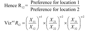
say we compare sites St and S2
If R12>1, then the outcome of location site S2 is better than the out-come of location I. In this manner we can get other pair wise comparisons and would be thus in a position to choose the best site.
Let us take an example.
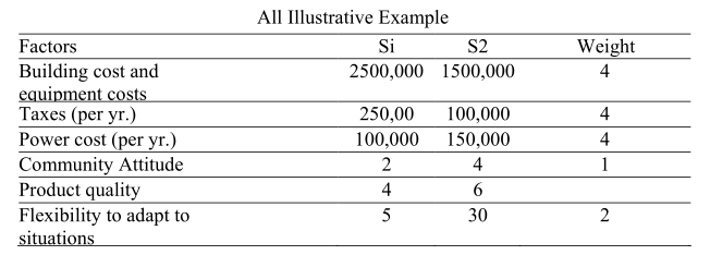
Hence R12
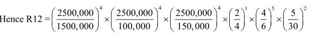
viz., R12 =0.02. As R12< 1, hence location site’ l is better-than location site 2 and is therefore selected.
