It is a mathematical optimization or feasibility program in which some or all of the variables are restricted to be integers. In many settings the term refers to integer linear programming (ILP), in which the objective function and the constraints (other than the integer constraints) are linear.
Integer programming algorithms minimize or maximize a linear function subject to equality, inequality, and integer constraints. Integer constraints restrict some or all of the variables in the optimization problem to take on only integer values. This enables accurate modeling of problems involving discrete quantities (such as shares of a stock) or yes-or-no decisions. Example integer programming problems include portfolio optimization in finance, optimal dispatch of generating units (unit commitment) in energy production, and scheduling and routing in operations research.
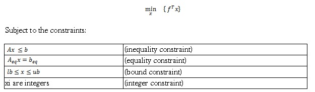
Integer programming requires finding a vector x that minimizes the function:
Solving such problems typically requires using a combination of techniques to narrow the solution space, find integer-feasible solutions, and discard portions of the solution space that do not contain better integer-feasible solutions. Common techniques include
- Cutting planes: Add additional constraints to the problem that reduce the search space.
- Heuristics: Search for integer-feasible solutions.
- Branch and bound: Systematically search for the optimal solution. The algorithm solves linear programming relaxations with restricted ranges of possible values of the integer variables.
Thus far we have been dealing with models in which the variables can take on real values, for example a solution value of 7.3 is perfectly fine. But the variables in some models are restricted to taking only integer or discrete values. You can assign 6 or 7 people to a team, for example, but not 6.3 people; or you can choose to make a transistor from silicon dioxide or gallium arsenide, but not some mixture. Binary variables are a subset of integer/discrete variables that are restricted to 0/1 values. Binary variables are usually associated with yes/no decisions, e.g. to undertake a project or not.
You will often encounter integer models that look like they can be solved by methods suitable for real-valued variables. For example, it is common to find models in which the objective function and constraints are linear relations defined on integer variables. This looks exactly like a standard linear program, except that the variables cannot take on real values. There is an overwhelming temptation to just solve the problem by standard linear programming and then to round any non-integer variable values to the closest integer value. Don’t do this! The following simple example (due to Hillier and Lieberman) shows how misleading this can be.
The linear programming solution to this problem yields Z=11 at (2, 1.8). The first instinct is to round x2 to the nearest integer value, i.e. x2=2. Unfortunately (2, 2) is infeasible by the first constraint. The natural inclination is then to try rounding x2 in the opposite direction, i.e. x2=1. This yields a feasible point (2, 1) with Z=7. However, this is not the optimum point! The integer-feasible optimum point is at (0, 2) where Z=10. Figure shows a sketch of this problem. The dots in figure show points at which both x1 and x2 have integer values simultaneously.
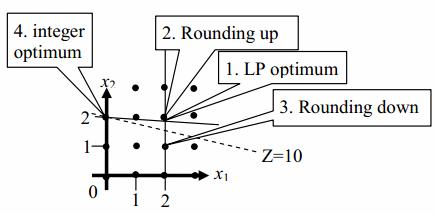
Notice that the integer optimum point is far away from the LP optimum. Notice also how you can’t get to the integer optimum (0,2) by rounding the LP optimum (2, 1.8). The moral of the story is that you simply can’t use real-valued solution methods to optimize integer-valued models. Completely different methods are needed.
The first thing you might think of for solving integer-valued problems is to simply enumerate all of the possible solutions and then to choose the best one. This will actually work for very small problems, but it very rapidly becomes unworkable for even small- to medium-size problems, let alone industrial-scale problems. For example, consider a binary 0/1 problem that has 20 variables. This will have 220 =1,048,576 solutions to enumerate, which might be possible to do via computer. Now consider a slightly larger binary problem having 100 variables. Now there are 2 100 =1.268 x 10 30 solutions to enumerate, which is likely impossible, even for a very fast computer. The combinatorial explosion is even worse for general integer variables that can take on even more values than just the two possibilities for binary variables. It is easy to construct problems in which the number of solutions is greater than the total number of atoms in the universe! Enumeration just won’t work for most real-world problems – we need a better way of tackling the combinatorial explosion.
The branch and bound method is the basic workhorse technique for solving integer and discrete programming problems. The method is based on the observation that the enumeration of integer solutions has a tree structure. For example, consider the complete enumeration of a model having one general integer variable x1, and two binary variables x2 and x3, whose ranges are 1≤ x1≤3, 0≤x2≤1, and 0≤ x3≤1. Figure below shows the complete enumeration of all of the solutions for these variables, even those which might be infeasible due to other constraints on the model.
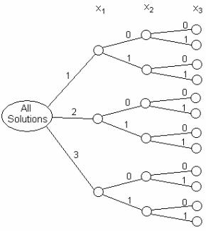
The structure in the figure looks like a tree lying on its side with the root (or root node) on the left, labeled “all solutions”, and the leaves (or leaf nodes) on the right. The leaf nodes represent the actual enumerated solutions, so there are 12 of them: (3 possible values of x1) x (2 possible values of x2) x (2 possible values of x3). For example, the node at the upper right represents the solution in which x1=1, x2=0, and x3=0. The other nodes can be thought of as representing sets of possible solutions. For example, the root node represents all solutions that can be generated by growing the tree. Another intermediate node, e.g. the first node directly to the right of the root node, represents another subset of all of the possible solutions, in this case, all of the solutions in which x1=2 and the other two variables can take on any of their possible values. For any two directly connected nodes in the tree, the parent node is the one closer to the root, and the child node is the one closer to the leaves.
Now the main idea in branch and bound is to avoid growing the whole tree as much as possible, because the entire tree is just too big in any real problem. Instead branch and bound grows the tree in stages, and grows only the most promising nodes at any stage. It determines which node is the most promising by estimating a bound on the best value of the objective function that can be obtained by growing that node to later stages. The name of the method comes from the branching that happens when a node is selected for further growth and the next generation of children of that node is created. The bounding comes in when the bound on the best value attained by growing a node is estimated. We hope that in the end we will have grown only a very small fraction of the full enumeration tree.
Another important aspect of the method is pruning, in which you cut off and permanently discard nodes when you can show that it, or any its descendents, will never be either feasible or optimal. The name derives from gardening, in which pruning means to clip off branches on a tree, exactly what we will do in this case. Pruning is one of the most important aspects of branch and bound since it is precisely what prevents the search tree from growing too much.
To describe branch and bound in detail, we first need to introduce some terminology
- Node: any partial or complete solution. For example, a node that is two levels down in a 5-variable problem might represent the partial solution 3-17-?-?-?, in which the first variable has a value of 3 and the second variable has a value of 17. The values of the last three variables are not yet set.
- Leaf (leaf node): a complete solution in which all of the variable values are known.
- Bud (bud node): a partial solution, either feasible or infeasible. Think of it as a node that might yet grow further, just as on a real tree.
- Bounding function: the method of estimating the best value of the objective function obtainable by growing a bud node further. Only bud nodes have associated bounding function values. Leaf nodes have objective function values, which are actual values and not estimates. It is important that the bounding function be an optimistic estimator. In other words, if you are minimizing, it must underestimate the actual best achievable objective function value; if maximizing it must overestimate the best achievable objective function value. You want it to be as accurate an estimator as possible so that the resulting branch and bound tree is as small as possible, but it must err in the optimistic direction. The bounding function is the real magic in branch and bound. It takes ingenuity sometimes to find a good bounding function, but the payoff in increased efficiency is tremendous. Every problem is different.
- Branching, growing, or expanding a node: the process of creating the child nodes for a bud node. One child node is created for each possible value of the next variable. For example, if the next variable is binary, there will be one child node associated with the value zero and one child node associated with the value one.
- Incumbent: the best complete feasible solution found so far. There may not be an incumbent when the solution process begins. In that case, the first complete feasible solution found during the solution process becomes the first incumbent.
The node selection policy governs how to choose the next bud node for expansion. There are three popular policies for node selection
- Best-first or global-best node selection: choose the bud node that has the best value of the bounding function anywhere on the branch and bound tree. If we are minimizing, this means choosing the bud node with the smallest value of the bounding function; if maximizing choose the bud node with the largest value of the bounding function.
- Depth-first: choose only from among the set of bud nodes just created. Choose the bud node with the best value of the bounding function. Depth-first node selection takes you one step deeper into the branch and bound tree at each iteration, so it reaches the leaf nodes quickly. This is one way of achieving an early incumbent solution. If you cannot proceed any deeper into the tree, back up one level and choose another child node from that level.
- Breadth-first: expand bud nodes in the same order in which they were created.
Similarly, once a bud node has been chosen for expansion, how do we choose the next variable to use in creating the child nodes of the bud node? The variable selection policy governs this choice. There are few standard policies for variable selection. The variables are often selected just in their natural order, though a good variable selection policy can improve efficiency greatly.
We also need to establish policies and rules for pruning bud nodes. As mentioned above, there are two main reasons to prune a bud node: you can show that no descendent will be feasible, or you can show that no descendent will be optimal.
The method for showing that no descendent will be optimal is standard: if the bud node bounding function value is worse than the objective function value for the incumbent, then the bud node can be pruned.
Methods for showing that no descendent can ever be feasible vary with the specific problem. There is one other case in which the expansion of a bud node can be halted: when the best possible value of the objective function obtainable by expansion can be seen directly. This is known as fathoming a node. Finally, we need a terminating rule to tell us when to stop expanding the branch and bound tree.
Example
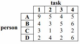
We have four persons, A through D, to assign to four tasks, 1 through 4. The table below shows the number of minutes it takes for each person to do each task. Each person can do exactly one task, and all tasks must have an assigned person. The objective is to minimize the total minutes taken. How many possible assignments of persons to tasks are there? There are 4!=24. In general, when there are n persons and n tasks there are n! possible assignments.
The formal branch and bound formulation follows. Any complete formulation must address all of these items.
- Meaning of a node in the branch and bound tree: a partial or complete assignment of
- persons to tasks. For example, a complete assignment ACBD represents the assignment of person A to task 1, person C to task 2, etc.
- Node selection policy: global best value of the bounding function.
- Variable selection policy: choose the next task in the natural order 1 to 4.
- Bounding function: for unassigned tasks, choose the best unassigned person, even if that person is chosen more than once. This is a relaxation of the original problem in which each person can do exactly one task.
- Terminating rule: when the incumbent solution objective function value is better than or equal to the bounding function values associated with all of the bud nodes.
- Fathoming: the “solution” generated by the bounding function is feasible if every task is assigned to a different person.
As an example of the calculation of the bounding function, let’s look at the first-level node associated with assigning person A to task 1. The set of solutions represented by this node is A???. The bounding function value is calculated as follows:
- Actual value associated with assigning A to task 1: 9.
- Best unassigned person for task 2 is C, value: 1.
- Best unassigned person for task 3 is D, value: 2.
- Best unassigned person for task 4 is C, value: 2.
- The bounding function “solution” is ACDC, with total cost = 9+1+2+2=14. At this point
- we know that the very best objective function value that we might find at a leaf node
- descended from A??? is 14. Since person C is repeated, this is not a feasible solution, so
- the node is not fathomed. Note that person A is actually assigned, so we will not see A
- repeated in the bounding function calculations at this node or at any of the descendent nodes
In practice, this bounding function amounts to crossing out the tasks (columns) that have assigned people, and the people (rows) that have assigned tasks, and then choosing the best number in each of the remaining columns, even if a particular person (row) is chosen more than once.
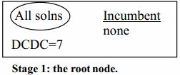
Now we are ready to develop the branch and bound tree. First we create the root node. It’s always worth finding the “solution” generated by the bounding function at the root node, since there is a chance that if you are fantastically lucky this “solution” will fathom the entire tree! Figure shows the root node. In all of the figures, each node is labeled with the “solution” generated by the bounding function, and the bounding function value. Pruned nodes are indicated by dashed borders, and feasible nodes are indicated by bold borders. Pruned feasible nodes have both features.
Below figure shows the next level of the tree, generated from the root node by enumerating the possible persons who can do task 1. Node C??? is fathomed, providing our first feasible solution and hence the first incumbent solution, CBDA=13. This allows us to prune node A??? whose bounding function value is 14.
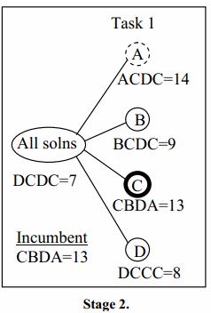
There are two bud nodes in stage 2 that show promise of improving on the incumbent solution: B??? with a bounding function value of 9 and D??? with a bounding function value of 8. Since we are using the global-best node selection policy, we choose node D??? for further expansion, which results in Stage 3. Note that the child nodes of D??? are labeled A, B, and C, but not D. Why? Because person D is already assigned, and so can’t be assigned again in descendent nodes. There are no new feasible solutions, so the incumbent solution is unchanged, and none of the new nodes can be pruned by comparison with the incumbent, or fathomed. So we choose the global best value of the bounding function between nodes B??? with value 9, DA?? with value 12, DB?? with value 10 and DC?? With value 12. The best of these is node B???, which is expanded in stage 4.
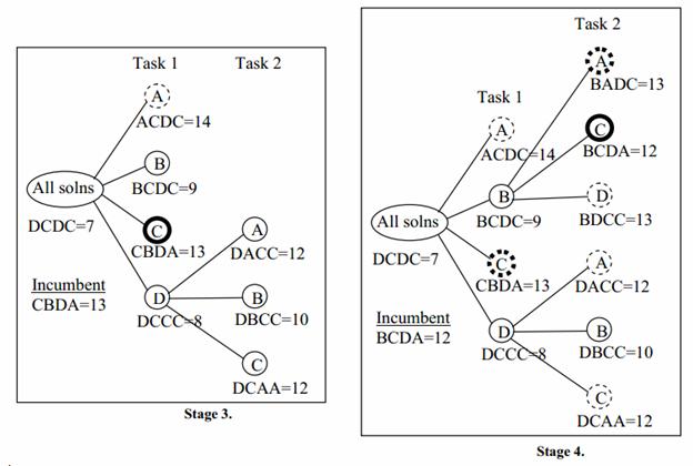
Stage 4 shows that there are two new fathomed nodes, BA?? and BC??. The feasible bounding function “solution” associated with BC?? has a lower value than the current incumbent, and so replaces it and prunes the old incumbent. Node BA??, even though feasible, is pruned by comparison with the new incumbent. Nodes DA?? and DC?? are also pruned by comparison with the incumbent (these could be kept for potential later exploration if we wanted to find all possible optimum solutions instead of just one). There remains only a single bud node which has the possibility of producing a better solution than the incumbent: node DB??. This node is expanded to produce stage 5.
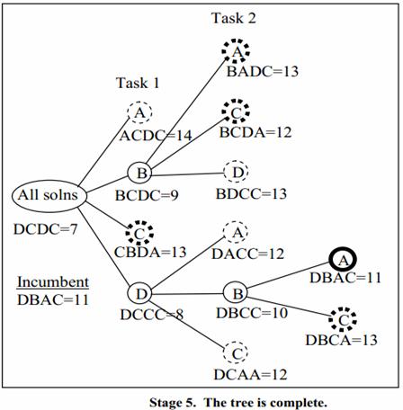
Stage 5 shows the expansion of DB?? to produce two child nodes. Both of these are feasible since once the first 3 persons are chosen, the only unassigned person is assigned to the final task, producing a feasible solution. The newly produced solution DBAC has a better objective function value than the incumbent, and so replaces it and prunes the old incumbent. The other newly created solution, DBCA, is pruned by comparison with the new incumbent. At this point there are no bud nodes remaining for possible expansion, so we stop. The final solution is given by the current incumbent: DBAC with a minimum total time of 11 minutes for the assignment.
Now how much work did we do? We evaluated 13 nodes, including the root node. This is about half of the work of a full enumeration of the 24 possible solutions, quite a good speed-up. However, branch and bound solutions for large problems should do a much smaller fraction of the work, more like a tenth of a percent or less.
Some final notes on branch and bound methodology. First, how do we deal with ties for the next node to choose for expansion? You can simply choose arbitrarily: if you choose wrongly, the branch and bound method will eventually bring you back to the unchosen node. A general rule of thumb is to first choose the node that is farthest away from the root, since it is more likely to be closer to a feasible solution.
Second, suppose the incumbent solution objective function value is tied with the bounding function value at some bud nodes. If we are only interested in a single solution to the problem, then the bud nodes can be pruned because the best that they can do is to eventually grow into solutions equal to the one we already have on hand, and even that is not very likely. On the other hand, if we are interested in finding all of the optimal solutions, then those bud nodes are kept until a strictly better incumbent solution prunes them. At the end, if there are bud nodes that have the same bounding function as the optimum solution, then they are explored: each will either produce a different solution with the same value of the objective function, or will be pruned. This allows us to generate all of the equivalent optimum solutions. In stage 5 we pruned two bud nodes that had bounding function values equal to the incumbent objective function value because we were interested in finding just one single optimum solution.
