Cyclomatic complexity is a software metric used to indicate the complexity of a program. It is a quantitative measure of the number of linearly independent paths through a program’s source code. It was developed by Thomas J. McCabe, Sr. in 1976.
Cyclomatic complexity is computed using the control flow graph of the program: the nodes of the graph correspond to indivisible groups of commands of a program, and a directed edge connects two nodes if the second command might be executed immediately after the first command. Cyclomatic complexity may also be applied to individual functions, modules, methods or classes within a program.
One testing strategy, called basis path testing by McCabe who first proposed it, is to test each linearly independent path through the program; in this case, the number of test cases will equal the cyclomatic complexity of the program.
Cyclomatic complexity of a code section is the quantitative measure of the number of linearly independent paths in it. It is a software metric used to indicate the complexity of a program. It is computed using the Control Flow Graph of the program. The nodes in the graph indicate the smallest group of commands of a program, and a directed edge in it connects the two nodes i.e. if second command might immediately follow the first command.
For example, if source code contains no control flow statement then its cyclomatic complexity will be 1 and source code contains a single path in it. Similarly, if the source code contains one if condition then cyclomatic complexity will be 2 because there will be two paths one for true and the other for false.
Mathematically, for a structured program, the directed graph inside control flow is the edge joining two basic blocks of the program as control may pass from first to second.
So, cyclomatic complexity M would be defined as,
M = E – N + 2P
where,
E = the number of edges in the control flow graph
N = the number of nodes in the control flow graph
P = the number of connected components
Steps that should be followed in calculating cyclomatic complexity and test cases design are:
- Construction of graph with nodes and edges from code.
- Identification of independent paths.
- Cyclomatic Complexity Calculation
- Design of Test Cases
An alternative formulation is to use a graph in which each exit point is connected back to the entry point. In this case, the graph is strongly connected, and the cyclomatic complexity of the program is equal to the cyclomatic number of its graph (also known as the first Betti number), which is defined as
M = E − N + P.
This may be seen as calculating the number of linearly independent cycles that exist in the graph, i.e. those cycles that do not contain other cycles within themselves. Note that because each exit point loops back to the entry point, there is at least one such cycle for each exit point.
For a single program (or subroutine or method), P is always equal to 1. So a simpler formula for a single subroutine is
M = E − N + 2.
Cyclomatic complexity may, however, be applied to several such programs or subprograms at the same time (e.g., to all of the methods in a class), and in these cases P will be equal to the number of programs in question, as each subprogram will appear as a disconnected subset of the graph.
Applications
Limiting complexity during development – One of McCabe’s original applications was to limit the complexity of routines during program development; he recommended that programmers should count the complexity of the modules they are developing, and split them into smaller modules whenever the cyclomatic complexity of the module exceeded 10. This practice was adopted by the NIST Structured Testing methodology, with an observation that since McCabe’s original publication, the figure of 10 had received substantial corroborating evidence, but that in some circumstances it may be appropriate to relax the restriction and permit modules with a complexity as high as 15. As the methodology acknowledged that there were occasional reasons for going beyond the agreed-upon limit, it phrased its recommendation as “For each module, either limit cyclomatic complexity to [the agreed-upon limit] or provide a written explanation of why the limit was exceeded.”
Measuring the “structuredness” of a program – Section VI of McCabe’s 1976 paper is concerned with determining what the control flow graphs (CFGs) of non-structured programs look like in terms of their subgraphs, which McCabe identifies. McCabe concludes that section by proposing a numerical measure of how close to the structured programming ideal a given program is, i.e. its “structuredness” using McCabe’s neologism. McCabe called the measure he devised for this purpose essential complexity.
In order to calculate this measure, the original CFG is iteratively reduced by identifying subgraphs that have a single-entry and a single-exit point, which are then replaced by a single node. This reduction corresponds to what a human would do if they extracted a subroutine from the larger piece of code. (Nowadays such a process would fall under the umbrella term of refactoring.) McCabe’s reduction method was later called condensation in some textbooks, because it was seen as a generalization of the condensation to components used in graph theory. If a program is structured, then McCabe’s reduction/condensation process reduces it to a single CFG node. In contrast, if the program is not structured, the iterative process will identify the irreducible part. The essential complexity measure defined by McCabe is simply the cyclomatic complexity of this irreducible graph, so it will be precisely 1 for all structured programs, but greater than one for non-structured programs.
Implications for software testing – Another application of cyclomatic complexity is in determining the number of test cases that are necessary to achieve thorough test coverage of a particular module.
It is useful because of two properties of the cyclomatic complexity, M, for a specific module:
- M is an upper bound for the number of test cases that are necessary to achieve a complete branch coverage.
- M is a lower bound for the number of paths through the control flow graph (CFG). Assuming each test case takes one path, the number of cases needed to achieve path coverage is equal to the number of paths that can actually be taken. But some paths may be impossible, so although the number of paths through the CFG is clearly an upper bound on the number of test cases needed for path coverage, this latter number (of possible paths) is sometimes less than M.
Example
Example :
IF A = 10 THEN
IF B > C THEN
A = B
ELSE
A = C
ENDIF
ENDIF
Print A
Print B
Print C
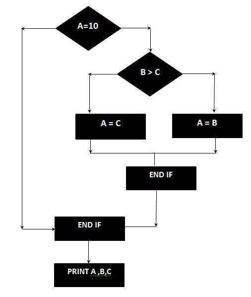
The Cyclomatic complexity is calculated using the above control flow diagram that shows seven nodes(shapes) and eight edges (lines), hence the cyclomatic complexity is 8 – 7 + 2 = 3
