Each parameter of a manufactured unit has opportunities for failure. The identification and measurement of these failures by basic six sigma metrics is essential.
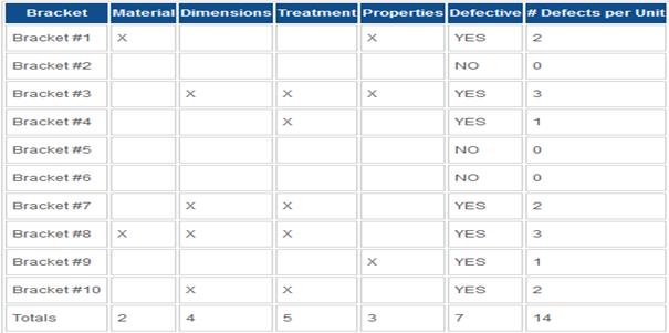
Let’s use an example of a stamped and anodized aluminum L-bracket with four features: material (aluminum), treatment (anodizing), dimensions, and required properties. The following chart will be used for each basic six sigma metric covered, as
Defects per Unit (DPU)
One way to understand how well a process performs is to identify the resulting Defects per Unit (i.e. the number of defects per manufactured unit). The chart identifies 10 total units produced. Of them, 7 are defective and there are 14 total defects. Note that almost all units have multiple defects. It is important to distinguish between these two concepts. A defect is an occurrence of non-conformance to customer requirements. A defective unit is a product with one or more defects or non-conformant features. It is possible for a single product to have multiple defects, as this chart suggests. The formula for Defects per Unit is:
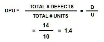
There are 1.4 Defects per Unit in this process.
Defects per Opportunity (DPO)
Defects per Opportunity describe the average defects (opportunities for defects) in each unit produced. This is not a hard count of the number of defects, but a measure of the probability of defects. DPO may be expressed by three separate formulae using similar data. They each depend on the data collected from the chart above:
D = # defects (14) TOP = total # of failure opportunities (40)
O = # defect opportunities (4) DPU = defects per unit (1.4)
U = # units (10)
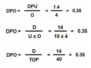
Either formula, using different data points, gives the same result for this process: the average number of defects, or the probability of defects, in each produced unit is 0.35 DPO.
Defects per Million Opportunities (DPMO)
Defects per million opportunities (DPMO) is also a probability measure. It calculates the probability that a given process will produce X defect opportunities per million units produced.2 One million units is used in the formula as a convenient constant, regardless of the actual number of units a process produces. The formula is:
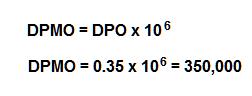
This formula uses the data from the previous metric, DPO. It differs from a calculation of (defective) Parts per Million (PPM) (will be discussed below) in that it accounts for the fact that there are multiple failure opportunities in a single manufactured unit. One should not assume that those opportunities automatically become actual failures. For the metric, DPMO, using the data from the chart above, there is a probability that there are 350,000 defect opportunities.
Parts per Million (PPM)
PPM counts the quantity of defective parts per million parts produced. As noted above, it does not account for the fact that multiple defects may affect a single part. One defective part, even with multiple defects, counts as a single defective among other defectives in the population. As with DPMO, it uses 1,000,000 as a constant, regardless of the actual number of parts produced. The formula is:
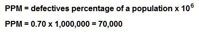
In our process example, 7 defective units (count the number of defectives, not the number of defects) of 10 units produced yields a PPM of 70,000.
First Pass Yield (FPY), or Throughput Yield (TPY), and First Time Yield (FTY), Rolled Throughput Yield (RTY)
First Pass Yield and Throughput Yield are synonymous terms that define the number of units successfully produced in a process step, i.e., without defects, divided by the total number of units entering that process. For example, using the chart above, of 10 units entering the stamping process to yield correct dimensions, 6 were defect-free products, or 6/10. To count as FPY/TPY units, they must pass completely through the process without rework or scrap.
The formula is simple:
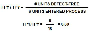
The First Pass Yield or Throughput Yield of the stamping process is 0.60, or 60 percent.
First Time Yield (FTY) is a calculation used to determine when the total number of acceptable product leaves the process when rework/scrap are counted, but only if the rework performed corrects the defect(s). Let’s assume that of the 5 treatment (anodizing) defects found, 4 are able to be reworked. This increases the number of acceptable units through that process by 4 units, or 7 acceptable units total. The formula is:
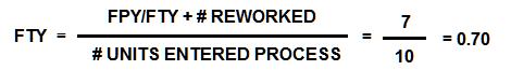
It is important to include only the successfully reworked product in the formula. The rework resulted in a First Time Yield of 0.70, or 70 percent.
Rolled Throughput Yield (RTY) is an accumulated total, by multiplication, of the results of all FPY/FTY-measured processes. In our example, we have four processes that produce a finished part: material, stamping, anodizing and properties. In the materials (verification) process, there are 2 failures in 10 units (FPY = 80 percent). In the stamping process, there are 4 failures in 10 units (FPY = 60 percent). In the anodizing process, there are 5 failures in 10 units (FPY = 50 percent). In the properties (verification) process, there are 3 failures in 10 units (FPY = 70 percent). The formula is:
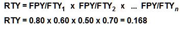
Our example indicates that the Rolled Throughput Yield (RTY) for all processes is only 16.8 percent.
Cycle Time, Manufacturing Lead Time, and TAKT Time
These three metrics are also critical to Six Sigma. They are not difficult to calculate, and in two cases, no formula is required.
Cycle Time is simply the time from beginning to completion of a process step. In our example, it might be the elapsed time in the stamping process from the retrieval of a raw material aluminum bar from an input bin, loading it into the press, cycling the press, removing the stamped part, and placing it into an output bin. Each of these segments can be measured separately, or the cumulative of all segments together, but they are timed by a stopwatch and recorded accordingly. Several measurements should be taken to arrive at an average cycle time for the process.
Manufacturing Lead Time is the measure of the total time to manufacture a part through its complete value stream, or entire manufacturing process. In our example, this would include both value-added and non-value-added time in process, calculated from the point of retrieval of raw material from the supplier delivery dock to the point of loading finished goods into a shipping truck. The stamping process noted above is just one segment of the value stream, which could even include the transport time of a single, or batch, of components from one internal process to the next, as well as delay time in storage between active process steps.
It is important to separate value-added activity (that is, any process activity that adds value to the in-process part) and non-value added activity (that is, any process activity that does not add value, such as transport and storage). For a more complete value stream, the order process, and delivery to the customer’s dock may be included.
TAKT Time (takt is German, meaning “pace,” or “rhythm”) is the calculated rate required to produce product within the time demanded by a customer order.5 If our L-bracket customer has ordered 10,000 brackets to be delivered in daily increments of 500, and we know we have 8 hours (480 minutes) to produce each daily batch, the formula to use is:
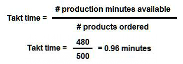
We have less than one minute of takt time to meet the customer demand. If it seems impossible to fully produce one bracket per minute (let alone less), we must recall that a series of processes like this example can produce multiple units in a batch, so the takt time is achievable.
