It is a statistical process for estimating the relationships among variables. It includes many techniques for modeling and analyzing several variables, when the focus is on the relationship between a dependent variable and one or more independent variables (or ‘predictors’). More specifically, regression analysis helps one understand how the typical value of the dependent variable (or ‘criterion variable’) changes when any one of the independent variables is varied, while the other independent variables are held fixed. Most commonly, regression analysis estimates the conditional expectation of the dependent variable given the independent variables – that is, the average value of the dependent variable when the independent variables are fixed.
For example, a businessperson may want to know whether the volume of sales for a given month is related to the amount of advertising the firm does that month.
Regression analysis is widely used for prediction and forecasting. Many techniques for carrying out regression analysis have been developed. Familiar methods such as linear regression and ordinary least squares regression are parametric, in that the regression function is defined in terms of a finite number of unknown parameters that are estimated from the data. Nonparametric regression refers to techniques that allow the regression function to lie in a specified set of functions, which may be infinite-dimensional.
The performance of regression analysis methods in practice depends on the form of the data generating process, and how it relates to the regression approach being used. Since the true form of the data-generating process is generally not known, regression analysis often depends to some extent on making assumptions about this process. These assumptions are sometimes testable if a sufficient quantity of data is available. Regression models for prediction are often useful even when the assumptions are moderately violated, although they may not perform optimally. However, in many applications, especially with small effects or questions of causality based on observational data, regression methods can give misleading results.
In a multiple relationship, called multiple regression, two or more independent variables are used to predict one dependent variable. For example, an educator may wish to investigate the relationship between a student’s success in college and factors such as the number of hours devoted to studying, the student’s GPA, and the student’s high school background. This type of study involves several variables.
Simple relationships can also be positive or negative. A positive relationship exists when both variables increase or decrease at the same time. For instance, a person’s height and weight are related; and the relationship is positive, since the taller a person is, generally, the more the person weighs. In a negative relationship, as one variable increases, the other variable decreases, and vice versa. For example, if you measure the strength of people over 60 years of age, you will find that as age increases, strength generally decreases. The word generally is used here because there are exceptions.
Simple Regression
In simple regression studies, the researcher collects data on two numerical or quantitative variables to see whether a relationship exists between the variables. For example, if a researcher wishes to see whether there is a relationship between number of hours of study and test scores on an exam, she must select a random sample of students, determine the hours each studied, and obtain their grades on the exam.
The two variables for this study are called the independent variable and the dependent variable. The independent variable is the variable in regression that can be controlled or manipulated. In this case, the number of hours of study is the independent variable and is designated as the x variable. The dependent variable is the variable in regression that cannot be controlled or manipulated. The grade the student received on the exam is the dependent variable, designated as the y variable. The reason for this distinction between the variables is that you assume that the grade the student earns depends on the number of hours the student studied. Also, you assume that, to some extent, the student can regulate or control the number of hours he or she studies for the exam.
The determination of the x and y variables is not always clear-cut and is sometimes an arbitrary decision. For example, if a researcher studies the effects of age on a person’s blood pressure, the researcher can generally assume that age affects blood pressure. Hence, the variable age can be called the independent variable, and the variable blood pressure can be called the dependent variable. On the other hand, if a researcher is studying the attitudes of husbands on a certain issue and the attitudes of their wives on the same issue, it is difficult to say which variable is the independent variable and which is the dependent variable. In this study, the researcher can arbitrarily designate the variables as independent and dependent.
The independent and dependent variables can be plotted on a graph called a scatter plot. The independent variable x is plotted on the horizontal axis, and the dependent variable y is plotted on the vertical axis.
Scatter Diagram
It displays multiple XY coordinate data points represent the relationship between two different variables on X and Y-axis. It is also called as correlation chart. It depicts the relationship strength between an independent variable on the vertical axis and a dependent variable on the horizontal axis. It enables strategizing on how to control the effect of the relationship on the process. It is also called scatter plots, X-Y graphs or correlation charts.
It graph pairs of continuous data, with one variable on each axis, showing what happens to one variable when the other variable changes. If the relationship is understood, then the dependent variable may be controlled. The relationship may show a correlation between the two variables though correlation does not always refer to a cause and effect relationship. The correlation may be positive due to one variable moving in one direction and the second variable in the same direction but, for negative correlation both move in opposite directions. Presence of correlation is due to a cause-effect relationship, a relationship between one cause and another cause or due to a relationship between one cause and two or more other causes.
It is used when two variables are related or evaluating paired continuous data. It is also helpful to identify potential root causes of a problem by relating two variables. The tighter the data points along the line, the stronger the relationship amongst them and the direction of the line indicates whether the relationship is positive or negative. The degree of association between the two variables is calculated by the correlation coefficient. If the points show no significant clustering, there is probably no correlation.
Correlation Coefficient
Statisticians use a measure called the correlation coefficient to determine the strength of the linear relationship between two variables. There are several types of correlation coefficients.
The correlation coefficient computed from the sample data measures the strength and direction of a linear relationship between two variables. The symbol for the sample correlation coefficient is r. The symbol for the population correlation coefficient is r (Greek letter rho).
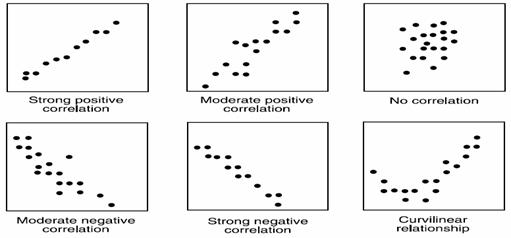
The range of the correlation coefficient is from -1 to +1. If there is a strong positive linear relationship between the variables, the value of r will be close to +1. If there is a strong negative linear relationship between the variables, the value of r will be close to -1. When there is no linear relationship between the variables or only a weak relationship, the value of r will be close to 0.
Formula for the Correlation Coefficient r
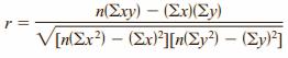
where n is the number of data pairs.
Example
Compute the correlation coefficient for car rental companies for a recent year.
| Company | Cars (in ten thousands) | Revenue (in billions) |
| A | 63.0 | $7.0 |
| B | 29.0 | 3.9 |
| C | 20.8 | 2.1 |
| D | 19.1 | 2.8 |
| E | 13.4 | 1.4 |
| F | 8.5 | 1.5 |
Step 1 Make a table as shown
| Company | Cars x (in ten thousands) | Income y (in billions) | xy | x2 | y2 |
| A | 63.0 | 7.0 | |||
| B | 29.0 | 3.9 | |||
| C | 20.8 | 2.1 | |||
| D | 19.1 | 2.8 | |||
| E | 13.4 | 1.4 | |||
| F | 8.5 | 1.5 |
Step 2 Find the values of xy , x2, and y2 and place these values in the corresponding columns of the table. The completed table is as
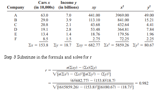
The correlation coefficient suggests a strong relationship between the number of cars a rental agency has and its annual income.
Population Correlation Coefficient
The population correlation coefficient is computed from taking all possible (x, y) pairs; it is designated by the Greek letter r (rho). The sample correlation coefficient can then be used as an estimator of r if the following assumptions are valid.
- The variables x and y are linearly related.
- The variables are random variables.
- The two variables have a bivariate normal distribution.
A biviarate normal distribution means that for the pairs of (x, y) data values, the corresponding y values have a bell-shaped distribution for any given x value, and the x values for any given y value have a bell-shaped distribution.
Formally defined, the population correlation coefficient r is the correlation computed by using all possible pairs of data values ( x, y) taken from a population.
Significance of the Correlation coefficient
In hypothesis testing, one of these is true:
H0: r equals 0 – This null hypothesis means that there is no correlation between the x and y variables in the population.
H1: r not equals 0 – This alternative hypothesis means that there is a significant correlation between the variables in the population.
When the null hypothesis is rejected at a specific level, it means that there is a significant difference between the value of r and 0. When the null hypothesis is not rejected, it means that the value of r is not significantly different from 0 (zero) and is probably due to chance.
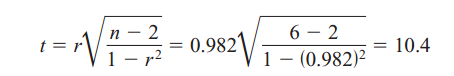
Several methods can be used to test the significance of the correlation coefficient like the t test, as

with degrees of freedom equal to n – 2.
Although hypothesis tests can be one-tailed, most hypotheses involving the correlation coefficient are two-tailed. Recall that r represents the population correlation coefficient.
Example
Test the significance of the correlation coefficient as per data given in earlier example
Step 1 – State the hypotheses.
H0 : r equals 0 and H1: r not equals 0
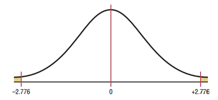
Step 2 – Find the critical values. Since = 0.05 and there are 6 – 2 = 4 degrees of freedom, the critical values obtained from Statistical table are +/-2.776, as shown below
Step 3 – Compute the test value.
Step 4 – Make the decision. Reject the null hypothesis, since the test value falls in the critical region, as shown
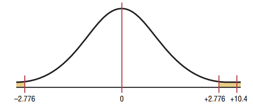
Step 5 – Summarize the results. There is a significant relationship between the number of cars a rental agency owns and its annual income.
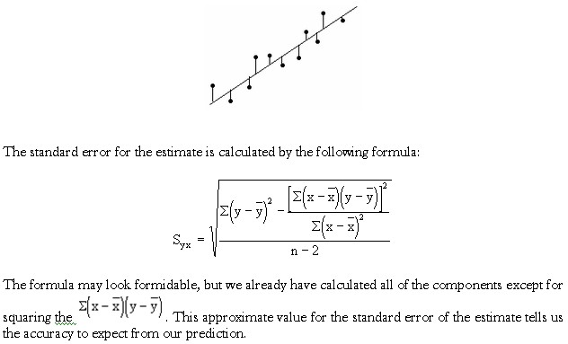
Standard Error of Estimate
The standard error of the estimate is a measure of the accuracy of predictions made with a regression line. The standard error of the estimate is a measure of the accuracy of predictions.
S represents the average distance that the observed values fall from the regression line. Conveniently, it tells you how wrong the regression model is on average using the units of the response variable. Smaller values are better because it indicates that the observations are closer to the fitted line. S becomes smaller when the data points are closer to the line.
It is the least squares estimator of a linear regression model with a single explanatory variable. In other words, simple linear regression fits a straight line through the set of n points in such a way that makes the sum of squared residuals of the model (that is, vertical distances between the points of the data set and the fitted line) as small as possible.
The adjective simple refers to the fact that the outcome variable is related to a single predictor. The slope of the fitted line is equal to the correlation between y and x corrected by the ratio of standard deviations of these variables. The intercept of the fitted line is such that it passes through the center of mass of the data points.
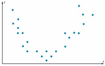
In studying relationships between two variables, collect the data and then construct a scatter plot. The purpose of the scatter plot, as indicated previously, is to determine the nature of the relationship. The possibilities include a positive linear relationship, a negative linear relationship, a curvilinear relationship, or no discernible relationship. After the scatter plot is drawn, the next steps are to compute the value of the correlation coefficient and to test the significance of the relationship. If the value of the correlation coefficient is significant, the next step is to determine the equation of the regression line, which is the data’s line of best fit. The purpose of the regression line is to enable the researcher to see the trend and make predictions on the basis of the data.
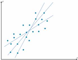
Line of Best Fit
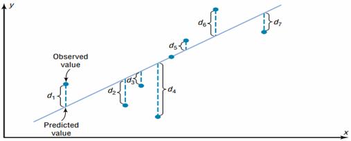
Given a scatter plot, you must be able to draw the line of best fit. Best fit means that the sum of the squares of the vertical distances from each point to the line is at a minimum.
Basic Equation for Regression – Observed Value = Fitted Value + Residual
The least squares line is the line that minimizes the sum of the squared residuals. It is the line quoted in regression outputs.
The reason you need a line of best fit is that the values of y will be predicted from the values of x; hence, the closer the points are to the line, the better the fit and the prediction will be. When r is positive, the line slopes upward and to the right. When r is negative, the line slopes downward from left to right.
A fitted value is the predicted value of the dependent variable. Graphically, it is the height of the line above a given explanatory value. The corresponding residual is the difference between the actual and fitted values of the dependent variable.
In algebra, the equation of a line is usually given as y = mx+ b, where m is the slope of the line and b is the y intercept. In statistics, the equation of the regression line is written as y’ = a + bx , where a is the y’ intercept and b is the slope of the line.
There are several methods for finding the equation of the regression line. These formulas use the same values that are used in computing the value of the correlation coefficient.
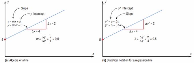
Formulas for the Regression Line y’ = a + bx
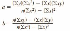
where a is the y’ intercept and b is the slope of the line.
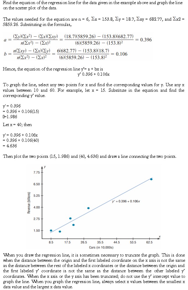
Example