One of the major operating difficulties in the scientific inventory control is an extremely large variety of items stocked by various organizations. These may vary from 10,000 to 100,000 different types of stocked items and it is neither feasible nor desirable to apply rigorous scientific principles of inventory control in all these items. Such an indiscriminate approach may make cost of inventory control more than its benefits and therefore may prove to be counter-productive. Therefore, inventory control has to be exercised selectively. Depending upon the value, criticality and usage frequency of an item we may have to decide on an appropriate type of inventory policy. The selective inventory management thus plays a crucial role so that we can put our limited control efforts more judiciously to the more significant group of items. In selective management we group items in few discrete categories depending upon value; criticality and usage frequency. Such analyses are popularly known as ABC, VED and FSN Analysis respectively. This type of grouping may well form the starting point in introducing scientific inventory management in an organization.
ABC Analysis
This is based on a very universal Pareto’s Law that in any large number we have `significant few’ and `insignificant many’. For example, only 20% of the items may be accounting for the 80% of the total material cost annually. These are the significant few which require utmost attention.
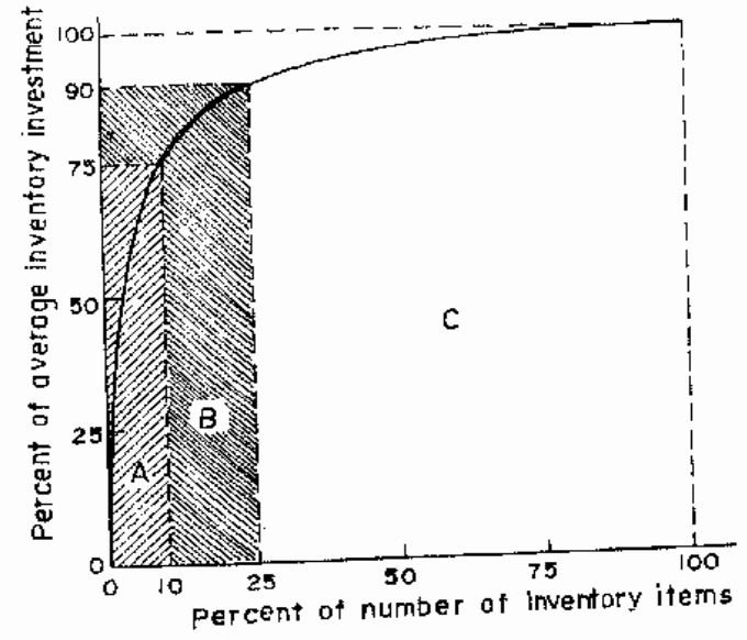
Figure IV shows a typical ABC analysis showing percentage of number of inventory items and percentage of average inventory investment (annual usage value). Annual usage value is the demand multiplied by unit price thus giving monetary worth of annual consumption. It can be seen from this figure that 10% items are claiming 75% of the annual usage value and thus constitute the `significant few’. These are called A-class items another 15% items account for another 15% annual usage value and are called B-class items. A vast majority of 75% items account for only 10% expenditure on material consumption and constitute `insignificant many’ and are called C-class items. To prepare an ABC type curve we may follow the following simple procedure:
- Arrange items in the descending order of the annual usage value. Annual usage value = Annual demand x Unit price.
- Identify cut off points on the curve when there is a perceptible sudden change o1 slope or alternatively find cut off points at top 10% next 20% or so but do not interpret these too literally- rather as a general indicator.
A very simple empirical way to classify items may be adopted as follows:
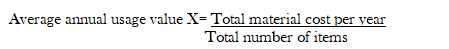
A-Class items ≤ 6X
C-Class items ≥ 0.5X
In between we have B-class items.
Once the items are grouped into A, B and C category, we can adopt different degree ‘ of seriousness in our inventory control efforts. A class items require almost continuous and rigorous control. Whereas B-class items may have relaxed control and C-class items may be procured using simple rules of thumb, as usual.
VED Analysis
This analysis attempts to classify items into three categories depending upon the consequences of material stock out when demanded. As stated earlier, the cost of shortage may vary depending upon the seriousness of such a situation. Accordingly the items are classified into V(Vital), E(Essential) and D(Desirable) categories. Vital items are the most critical having extremely high opportunity cost of shortage and must be available in stock when demanded. Essential items are quite critical with substantial cost associated with shortage and should be available in stock by and large. Desirable group of items do not have very serious consequences if not available when demanded but can be stocked items.
Obviously the % risk of shortage with the `vital’ group of items has to be quite small-thus calling for a high level of service. With `Essential’ category we can take a relatively higher risk of shortage and for `Desirable’ category even higher. Since even a C-class item may be vital or an A-class item may be `Desirable’ we should carry out a two-way classification of items grouping them in 9 distinct groups as A-V, A-E, A-D, B-V, B-E, B-D, C-V, C-E and C.D. Then we are able to argue on the aimed at service-level for each of these nine categories and plan for inventories accordingly.
FSN Analysis
Not all items are required with the same frequency. Some materials are quite regularly required, yet some others are required very occasionally and some materials may have become obsolete and might not have been demanded for years together. FSN analysis groups them into three categories as Fast-moving, Slow-moving and Non-moving (dead stock) respectively. Inventory policies and models for the three categories have to be different. Most inventory models in literature are valid for the fast-moving items exhibiting a regular movement (consumption) pattern. Many spare parts come under the slow moving category which has to be managed on a different basis. For non-moving dead stock, we have to determine optimal stock disposal rules rather than inventory provisioning rules. Categorization of materials into these three types on value, criticality and usage enables us to adopt the right type of inventory policy to suit a particular situation. In this unit, we shall mainly be developing some decision models more appropriate for A-class and fast-moving items. Later on a brief discussion on the inventory management of slow-moving items will be given.
Activity A
- Collect consumption data for 100 different items for an organization and classify these into an ABC framework following the procedure described.
- List these items in a two-way classification ABC and VED and identify the number of items belonging to each of these 9 distinct groups.
