Regression analysis is a statistical process for estimating the relationships among variables. It includes many techniques for modeling and analyzing several variables, when the focus is on the relationship between a dependent variable and one or more independent variables. More specifically, regression analysis helps one understand how the typical value of the dependent variable (or ‘criterion variable’) changes when any one of the independent variables is varied, while the other independent variables are held fixed. Most commonly, regression analysis estimates the conditional expectation of the dependent variable given the independent variables – that is, the average value of the dependent variable when the independent variables are fixed. Less commonly, the focus is on a quantile, or other location parameter of the conditional distribution of the dependent variable given the independent variables. In all cases, the estimation target is a function of the independent variables called the regression function. In regression analysis, it is also of interest to characterize the variation of the dependent variable around the regression function which can be described by a probability distribution.
Regression analysis is widely used for prediction and forecasting, where its use has substantial overlap with the field of machine learning. Regression analysis is also used to understand which among the independent variables are related to the dependent variable, and to explore the forms of these relationships. In restricted circumstances, regression analysis can be used to infer causal relationships between the independent and dependent variables. However this can lead to illusions or false relationships, so caution is advisable; for example, correlation does not imply causation.
Many techniques for carrying out regression analysis have been developed. Familiar methods such as linear regression and ordinary least squares regression are parametric, in that the regression function is defined in terms of a finite number of unknown parameters that are estimated from the data. Nonparametric regression refers to techniques that allow the regression function to lie in a specified set of functions, which may be infinite-dimensional.
The performance of regression analysis methods in practice depends on the form of the data generating process, and how it relates to the regression approach being used. Since the true form of the data-generating process is generally not known, regression analysis often depends to some extent on making assumptions about this process. These assumptions are sometimes testable if a sufficient quantity of data is available. Regression models for prediction are often useful even when the assumptions are moderately violated, although they may not perform optimally. However, in many applications, especially with small effects or questions of causality based on observational data, regression methods can give misleading results.
Regression Models
Regression models involve the following variables
- The unknown parameters, denoted as β, which may represent a scalar or a vector.
- The independent variables, X.
- The dependent variable, Y.
In various fields of application, different terminologies are used in place of dependent and independent variables. A regression model relates Y to a function of X and β.
The approximation is usually formalized as E(Y | X) = f(X, β). To carry out regression analysis, the form of the function f must be specified. Sometimes the form of this function is based on knowledge about the relationship between Y and X that does not rely on the data. If no such knowledge is available, a flexible or convenient form for f is chosen.
Assume now that the vector of unknown parameters β is of length k. In order to perform a regression analysis the user must provide information about the dependent variable Y
- If N data points of the form (Y, X) are observed, where N < k, most classical approaches to regression analysis cannot be performed: since the system of equations defining the regression model is underdetermined, there are not enough data to recover β.
- If exactly N = k data points are observed, and the function f is linear, the equations Y = f(X, β) can be solved exactly rather than approximately. This reduces to solving a set of N equations with N unknowns (the elements of β), which has a unique solution as long as the X are linearly independent. If f is nonlinear, a solution may not exist, or many solutions may exist.
- The most common situation is where N > k data points are observed. In this case, there is enough information in the data to estimate a unique value for β that best fits the data in some sense, and the regression model when applied to the data can be viewed as an overdetermined system in β.
In the last case, the regression analysis provides the tools for
- Finding a solution for unknown parameters β that will, for example, minimize the distance between the measured and predicted values of the dependent variable Y (also known as method of least squares).
- Under certain statistical assumptions, the regression analysis uses the surplus of information to provide statistical information about the unknown parameters β and predicted values of the dependent variable Y.
Necessary number of independent measurements
Consider a regression model which has three unknown parameters, β0, β1, and β2. Suppose an experimenter performs 10 measurements all at exactly the same value of independent variable vector X (which contains the independent variables X1, X2, and X3). In this case, regression analysis fails to give a unique set of estimated values for the three unknown parameters; the experimenter did not provide enough information. The best one can do is to estimate the average value and the standard deviation of the dependent variable Y. Similarly, measuring at two different values of X would give enough data for a regression with two unknowns, but not for three or more unknowns.
If the experimenter had performed measurements at three different values of the independent variable vector X, then regression analysis would provide a unique set of estimates for the three unknown parameters in β.
In the case of general linear regression, the above statement is equivalent to the requirement that the matrix XTX is invertible.
Statistical Assumptions
When the number of measurements, N, is larger than the number of unknown parameters, k, and the measurement errors εi are normally distributed then the excess of information contained in (N − k) measurements is used to make statistical predictions about the unknown parameters. This excess of information is referred to as the degrees of freedom of the regression.
Underlying Assumptions
Classical assumptions for regression analysis include
- The sample is representative of the population for the inference prediction.
- The error is a random variable with a mean of zero conditional on the explanatory variables.
- The independent variables are measured with no error. (Note: If this is not so, modeling may be done instead using errors-in-variables model techniques).
- The predictors are linearly independent, i.e. it is not possible to express any predictor as a linear combination of the others.
- The errors are uncorrelated, that is, the variance–covariance matrix of the errors is diagonal and each non-zero element is the variance of the error.
- The variance of the error is constant across observations (homoscedasticity). If not, weighted least squares or other methods might instead be used.
These are sufficient conditions for the least-squares estimator to possess desirable properties; in particular, these assumptions imply that the parameter estimates will be unbiased, consistent, and efficient in the class of linear unbiased estimators. It is important to note that actual data rarely satisfies the assumptions. That is, the method is used even though the assumptions are not true. Variation from the assumptions can sometimes be used as a measure of how far the model is from being useful. Many of these assumptions may be relaxed in more advanced treatments. Reports of statistical analyses usually include analyses of tests on the sample data and methodology for the fit and usefulness of the model.
Assumptions include the geometrical support of the variables. Independent and dependent variables often refer to values measured at point locations. There may be spatial trends and spatial autocorrelation in the variables that violate statistical assumptions of regression. Geographic weighted regression is one technique to deal with such data. Also, variables may include values aggregated by areas. With aggregated data the modifiable a real unit problem can cause extreme variation in regression parameters. When analyzing data aggregated by political boundaries, postal codes or census areas results may be very distinct with a different choice of units.
Simple Regression
It is the least squares estimator of a linear regression model with a single explanatory variable. In other words, simple linear regression fits a straight line through the set of n points in such a way that makes the sum of squared residuals of the model (that is, vertical distances between the points of the data set and the fitted line) as small as possible.
The adjective simple refers to the fact that this regression is one of the simplest in statistics. The slope of the fitted line is equal to the correlation between y and x corrected by the ratio of standard deviations of these variables. The intercept of the fitted line is such that it passes through the center of mass (x, y) of the data points.
Other regression methods besides the simple ordinary least squares (OLS) also exist (see linear regression model). In particular, when one wants to do regression by eye, one usually tends to draw a slightly steeper line, closer to the one produced by the total least squares method. This occurs because it is more natural for one’s mind to consider the orthogonal distances from the observations to the regression line, rather than the vertical ones as OLS method does.
When the input and output variables are both continuous and to see a relationship between the two variables, regression and correlation are used. Determining how the predicted or dependent variable (the response variable, the variable to be estimated) reacts to the variations of the predicator or independent variable (the variable that explains the change) involves first to determine any relationship between them and it’s importance. Regression analysis builds a mathematical model that helps making predictions about the impact of variable variations.
Usually, there is more than one independent variable causing variations of a dependent variable like changes in the volume of cars sold depends on the price of the cars, the gas mileage, the warranty, etc. But the importance of all these factors in the variation of the dependent variable (the number of cars sold) is disproportional. Hence, project team should concentrate on one important factor instead of analyzing all the competing factors.
In simple linear regression, prediction of scores on one variable is done from the scores on a second variable. The variable to predict is called the criterion variable and is referred to as Y. The variable to base predictions on is called the predictor variable and is referred to as X. When there is only one predictor variable, the prediction method is called simple regression. In simple linear regression, the predictions of Y when plotted as a function of X form a straight line.
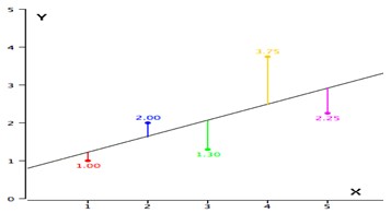
As an example, data for X and Y are listed below and having a positive relationship between X and Y. For predicting Y from X, the higher the value of X, the higher prediction of Y.
| X | Y |
| 1.00 | 1.00 |
| 2.00 | 2.00 |
| 3.00 | 1.30 |
| 4.00 | 3.75 |
| 5.00 | 2.25 |
Linear regression consists of finding the best-fitting straight line through the points. The best-fitting line is called a regression line. The diagonal line in the figure is the regression line and consists of the predicted score on Y for each possible value of X. The vertical lines from the points to the regression line represent the errors of prediction. As the line from 1.00 is very near the regression line; its error of prediction is small and similarly for the line from 1.75 is much higher than the regression line and therefore its error of prediction is large.
Fitting the Regression Line
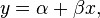
Suppose there are n data points {(xi, yi), i = 1, …, n}. The function that describes x and y is
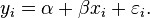
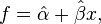
The goal is to find the equation of the straight line
which would provide a “best” fit for the data points. Here the “best” will be understood as in the least-squares approach: a line that minimizes the sum of squared residuals of the linear regression model. In other words, α (the y-intercept) and β (the slope) solve the following minimization problem:

By using either calculus, the geometry of inner product spaces, or simply expanding to get a quadratic expression in α and β, it can be shown that the values of α and β that minimize the objective function Q are
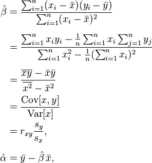
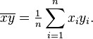
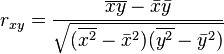
where rxy is the sample correlation coefficient between x and y; sx is the standard deviation of x; and sy is correspondingly the standard deviation of y. A horizontal bar over a quantity indicates the sample-average of that quantity. For example:
Substituting the above expressions for α and β into
yields
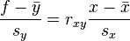
This shows the role rxy plays in the regression line of standardized data points. It is sometimes useful to calculate rxy from the data independently using this equation:
The coefficient of determination (R squared) is equal to when the model is linear with a single independent variable.
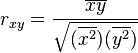
Linear regression without the intercept term
Sometimes, people consider a simple linear regression model without the intercept term, y = βx. In such a case, the OLS estimator for β simplifies to
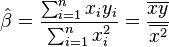
and the sample correlation coefficient becomes
Multiple Regression
The general purpose of multiple regression (the term was first used by Pearson, 1908) is to learn more about the relationship between several independent or predictor variables and a dependent or criterion variable. For example, a real estate agent might record for each listing the size of the house (in square feet), the number of bedrooms, the average income in the respective neighborhood according to census data, and a subjective rating of appeal of the house. Once this information has been compiled for various houses it would be interesting to see whether and how these measures relate to the price for which a house is sold. For example, you might learn that the number of bedrooms is a better predictor of the price for which a house sells in a particular neighborhood than how “pretty” the house is (subjective rating). You may also detect “outliers,” that is, houses that should really sell for more, given their location and characteristics.
Personnel professionals customarily use multiple regression procedures to determine equitable compensation. You can determine a number of factors or dimensions such as “amount of responsibility” (Resp) or “number of people to supervise” (No_Super) that you believe to contribute to the value of a job. The personnel analyst then usually conducts a salary survey among comparable companies in the market, recording the salaries and respective characteristics (i.e., values on dimensions) for different positions. This information can be used in a multiple regression analysis to build a regression equation of the form:
Salary = .5*Resp + .8*No_Super
Once this so-called regression line has been determined, the analyst can now easily construct a graph of the expected (predicted) salaries and the actual salaries of job incumbents in his or her company. Thus, the analyst is able to determine which position is underpaid (below the regression line) or overpaid (above the regression line), or paid equitably.
In the social and natural sciences multiple regression procedures are very widely used in research. In general, multiple regression allows the researcher to ask (and hopefully answer) the general question “what is the best predictor of …”. For example, educational researchers might want to learn what are the best predictors of success in high-school. Psychologists may want to determine which personality variable best predicts social adjustment. Sociologists may want to find out which of the multiple social indicators best predict whether or not a new immigrant group will adapt and be absorbed into society.
Multiple linear regression expands on the simple linear regression model to allow for more than one independent or predictor variable. The general form for the equation is y = b0+ b1x + … bn+ e where, (b0,b1,b2…) are the coefficients and are referred to as partial regression coefficients. The equation may be interpreted as the amount of change in y for each unit increase in x (variable) when all other xs are held constant. The hypotheses for multiple regression are Ho:b1=b2= … =bn Ha:b1≠ 0 for at least one i.
It is an extension of linear regression to more than one independent variable so a higher proportion of the variation in Y may be explained as first-order linear model

And second-order linear model

R2 the multiple coefficient of determination has values in the interval 0<=R2<=1
| Source | DF | SS | MS |
| Regression | k | SSR | MSR=SSR/k |
| Error | n-(k+1) | SSE | MSE=SSE[n-(k+1)] |
| Total | n-1 | Total SS |
Where k is the number of predictor variables.
Logistic Regression
Logistic regression, or logit regression, or logit model is a type of probabilistic statistical classification model. It is also used to predict a binary response from a binary predictor, used for predicting the outcome of a categorical dependent variable (i.e., a class label) based on one or more predictor variables (features). That is, it is used in estimating the parameters of a qualitative response model. The probabilities describing the possible outcomes of a single trial are modeled, as a function of the explanatory (predictor) variables, using a logistic function. Frequently (and hereafter in this article) “logistic regression” is used to refer specifically to the problem in which the dependent variable is binary—that is, the number of available categories is two—while problems with more than two categories are referred to as multinomial logistic regression or, if the multiple categories are ordered, as ordered logistic regression.
Logistic regression measures the relationship between the categorical dependent variable and one or more independent variables, which are usually (but not necessarily) continuous, by using probability scores as the predicted values of the dependent variable. Thus, it treats the same set of problems as does probit regression using similar techniques; the first assumes a logistic function and the second a standard normal distribution function.
Logistic regression can be seen as a special case of generalized linear model and thus analogous to linear regression. The model of logistic regression, however, is based on quite different assumptions (about the relationship between dependent and independent variables) from those of linear regression. In particular the key differences of these two models can be seen in the following two features of logistic regression. First, the conditional mean![]() follows a Bernoulli distribution rather than a Gaussian distribution, because logistic regression is a classifier. Second, the linear combination of the inputs
follows a Bernoulli distribution rather than a Gaussian distribution, because logistic regression is a classifier. Second, the linear combination of the inputs![]() is restricted to [0,1] through the logistic distribution function because logistic regression predicts the probability of the instance being positive.
is restricted to [0,1] through the logistic distribution function because logistic regression predicts the probability of the instance being positive.
Logistic regression can be binomial or multinomial. Binomial or binary logistic regression deals with situations in which the observed outcome for a dependent variable can have only two possible types (for example, “dead” vs. “alive”). Multinomial logistic regression deals with situations where the outcome can have three or more possible types (e.g., “disease A” vs. “disease B” vs. “disease C”). In binary logistic regression, the outcome is usually coded as “0” or “1”, as this leads to the most straightforward interpretation. If a particular observed outcome for the dependent variable is the noteworthy possible outcome (referred to as a “success” or a “case”) it is usually coded as “1” and the contrary outcome (referred to as a “failure” or a “noncase”) as “0”. Logistic regression is used to predict the odds of being a case based on the values of the independent variables (predictors). The odds are defined as the probability that a particular outcome is a case divided by the probability that it is a noncase.
Like other forms of regression analysis, logistic regression makes use of one or more predictor variables that may be either continuous or categorical data. Unlike ordinary linear regression, however, logistic regression is used for predicting binary outcomes of the dependent variable (treating the dependent variable as the outcome of a Bernoulli trial) rather than a continuous outcome. Given this difference, it is necessary that logistic regression take the natural logarithm of the odds of the dependent variable being a case (referred to as the logit or log-odds) to create a continuous criterion as a transformed version of the dependent variable. Thus the logit transformation is referred to as the link function in logistic regression—although the dependent variable in logistic regression is binomial, the logit is the continuous criterion upon which linear regression is conducted.
The logit of success is then fitted to the predictors using linear regression analysis. The predicted value of the logit is converted back into predicted odds via the inverse of the natural logarithm, namely the exponential function. Thus, although the observed dependent variable in logistic regression is a zero-or-one variable, the logistic regression estimates the odds, as a continuous variable, that the dependent variable is a success (a case). In some applications the odds are all that is needed. In others, a specific yes-or-no prediction is needed for whether the dependent variable is or is not a case; this categorical prediction can be based on the computed odds of a success, with predicted odds above some chosen cutoff value being translated into a prediction of a success.
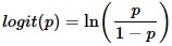
The goal of logistic regression is to find the best fitting (yet biologically reasonable) model to describe the relationship between the dichotomous characteristic of interest (dependent variable = response or outcome variable) and a set of independent (predictor or explanatory) variables. Logistic regression generates the coefficients (and its standard errors and significance levels) of a formula to predict a logit transformation of the probability of presence of the characteristic of interest

where p is the probability of presence of the characteristic of interest. The logit transformation is defined as the logged odds:

and
Rather than choosing parameters that minimize the sum of squared errors (like in ordinary regression), estimation in logistic regression chooses parameters that maximize the likelihood of observing the sample values.
