There are two types of estimates of current demand which may be helpful to a company. These are total market potential and territory potential. Total market potential is the maximum amount of sales that might be available to all the firms in an industry during a given period under a given level of industry marketing effort and given environmental conditions.
Where Q= total market potential
N= number of buyers in the specific product/ market under the given assumption.
Q= quantity purchased by an average buyer
P= price of an average unit
Of the components n.q and p in the above formula, the most difficult component to estimate is q. one can start with a broad concept of q, gradually reducing it. For example, if we are thinking of readymade shirts for him consumption, we may first take the total male population eliminating that in rural areas. From the total male urban population, we may eliminate the age groups which are not likely to buy readymade shirts. Thus, the number of boys below 20 may be eliminated. Further eliminations on account of low income may be made. In this way we can arrive at the prospect pool of those who are likely to but shirts.
The concept of market potential is helpful to the firm as it provides a benchmark against which actual performance can be measured. In addition, it can used as a basis for allocation decisions regarding marketing effort.
The estimate of total market potential is helpful to the company when it is in a dilemma whether to introduce a new product or drop an existing one. Such an estimate will indicate whether the prospective market is large enough to justify the company entering it .
Since it is impossible for a company to have the global market exclusively to itself, it has to select those territories where it can sell its products well. This means that companies should know the territorial potentials so that they can select markets most suited to them, channelise their marketing effort optimally among these markets and also evaluate their sale performance in such markets. There are two methods for estimating territorial potential:
- Market buildup method and
- Index –of –buying – power method. In the first method, several steps are involved. First, identify all the potential buyers for the product in each market. Second estimate potential purchases by each potential buyer.
- Third, sum up the individual figures in step (ii) above. However, in reality the estimation is not that simple as it is difficult to identify all potential buyers. When the product in question is an industrial, product, directories of manufactures of a particular product or group of products or groups alternatively, the standard industrial classification if manufacturers of a particular product or group of products are used.
The second method involves the use of a straight forward index. Suppose a textile manufacturing company is interested in knowing the territorial potential for its cloth in a certain territory. Symbolically,
Bi=0.5 Yi+ 0.2ri + 0.3pi
Bi=percentage of total national buying power in territory i.
Yi=percentage of national disposable personal originating in territory i. ri=percentage of national retail sales in territory i. It may be noted that be noted that such estimates indicate potential for the industry as a whole rather than for to individual company. In order to arrive at a company potential, the concerned company has to make certain adjustments in the above estimate on the basis of one or more other factors that have not been covered in the estimation of territorial potential. These factors could be the company’s brand share, number of salespersons, number and type of competitions, etc.
Forecasting Process: After having described the methods of estimating the current demand, we now turn to forecasting.
There are five steps involved in the forecasting process. These are mentioned below:
First, one has to decide the objective of the forecast. The marketing researcher should know as to what will be the use of the forecast he is going to make.
Second, the time period for which the forecast is to be made should be selected. Is there forecast short-term, medium-term or long-term?
Why should a particular period of forecast be selected?
Third, the method or technique or forecasting should be selected. One should be clear as to why a particular technique from amongst several techniques should be used.
Fourth, the necessary date should be collected. The need in specific data will depend on the forecasting technique to be used. Finally: the forecast is to be made. This will involve the use fo computational procedures.
In order to ensure that the forecast is really useful to the company, there should be good understanding between management and research. The management should clearly spell out the purpose of the forecast and how it is going to help the company. It should also ensure that the researcher has a proper understanding of the operations of the company. It environment, past performance in terms of key indicators and their relevance to the future trend. If the researcher is well-informed with respect to these aspects, then he is likely to make a more realistic and more useful forecast for the management.
Methods of Forecasting: The methods of forecasting can be divided into two broad categories, viz. subjective or qualitative methods and objective or quantitative methods. These can be further divided into several methods. Each of these methods is discussed below.
Subjective Methods: There are four subjective methods—field sales force, jury of executives, users’ expectation and Delphi. These are discussed here briefly.
Field Sales Force: Some companies ask their salesmen to indicate the most likely sales for a specified period in the future. Usually the salesman is asked to indicate anticipated sales for each account in his territory. These forecasts are checked by district managers who forward them to the company’s head office. Different territory forecasts are then combined into a composite forecast at the head office. This method is more suitable when a short-term forecast is to be made as there would be no major changes in this short period affecting the forecast. Another advantage of this method is that it involves the entire sales force which realizes its responsibility to achieve the target it has set for itself. A major limitation of this method is that sales force would not take an overall or board perspective and hence may overlook some vital factors influencing the sales. Another limitation is that salesmen may give somewhat low figures in their forecasts thing in that it may be easier for them to achieve those targets However, this can be offset to a certain extent by district managers who are supposed to check the forecasts.
Jury of Executives: Some companies prefer to assign the task of sales forecasting to executives instead of a sales force. Given this task each executive makes his forecast for the next period. Since each has his own assessment of the environment and other relevant factors, one forecast is likely to be different from the other. In view of this, it becomes necessary to have an average of these varying forecasts. Alternatively, steps should be taken to narrow down the difference in the forecasts. Sometimes this is done by organizing a discussion between the executives so that they can arrive at a common forecast. In case this is not possible, the chief executives so that they can arrive at a common forecast In case this is not possible, the chief executive may have to decide which of these forecasts is acceptable as a representative one.
This method is simple, At the same time, it is based on a number of different view points as opinions of different executives are sought. One major limitation of this method is that the executive’ opinions are likely to be influenced in one direction on the basis of general business conditions.
Users’ Expectations: Forecasts can be based on users’ expectations or intention to purchase goods and services. It is difficult to use this method when the number of users is large. Another limitation of this method is that though it indicates users’ ‘intention’ to buy, the actual purchases may be far less at a subsequent period. It is most suitable when the number of buyers is small such as in case of industrial products. The Delphi Method This method too is based on the experts’ opinions. Here, each expert has access to the same information that is available. A feedback system generally keeps them informed of each other’ forecasts but no majority opinion is disclosed to them. However, the experts are not brought together. This is to ensure that one or more vocal experts do not dominate other experts.
The experts are given an opportunity to compare their own previous forecasts with those of the others and revise them. After three or four rounds, the group of experts arrives at a final forecast.
The method may involve a large number of experts and this may delay the forecast considerably, generally it involves a small number of participants ranging from
It will be seen that both the jury of executive opinion and the Delphi method are based on a group of experts. They differ in that in the future, the group of experts meet, discuss the forecasts, and try to arrive at a commonly agreed while in the latter the group of experts never meets. As mentioned earlier, this is to one person dominates the discussion thus influencing the forecast. In other words, the Delphi method retains the wisdom of a group and at the same time reduces the effect of group pressure, An appropriate when long-term forecasts are involved.
In the subjected methods, judgment is an important ingredient. Before attempting a forecast, the basic assumptions regarding environmental conditions as also competitive behaviour must be provided to people involved in forecasting. An important advantage of subjective methods is that they are easily understood. Another advantage is that the cost involved in forecasting is quite low.
As against these advantages, subjective methods have certain limitations also. One major limitation is the varying perceptions of people involved in forecasting. As a result, wide variance is found in forecasts. Subjective methods are suitable when forecasts are to be made for highly technical products which have a limited number of customers. Generally such methods are used for industrial products. Also, when cost of forecasting is to be kept minim, subjective methods may be more suitable.
Quantitative or Statistical Methods: Based on statistical analysis, these methods enable the researcher to make forecasts on a more objective basis. It is difficult to make a wholly accurate forecast for there is always an element of uncertainty regarding the future. Even so, statistical methods are likely to be more useful as they are more scientific and hence more objective.
Time Series: In time-series forecasting, the past sales data are extrapolated as a linear or a curvilinear trend. Even if such data are plotted on a graph, on can extrapolate for the desire time period Extrapolation can also be made with the help of statistical techniques. It may be noted that time-series forecasting is most suitable to stable situations where the future trends will largely be an extension of the past. Further, the past sales data should have distinctive tends from the random error component for a time-series forecasting to be suitable.
Before using the time-series forecasting one has to decide how far back in the past one can go. It may be desirable to use the more recent data as conditions might have been different in the remote past. Another issue pertains to weighing of time-series data. In other words, should equal weight be given to each time period or should greater weightage be given to more recent data? Finally, should the data be decomposed into different components, viz. trend, cycle, season and error? We now discuss three methods, viz, moving averages, exponential smoothing and decomposition of time series.
Moving Average: This method used the last ‘n’ data points to compute a series of average in such a way that each time the latest figure is used and the earliest one dropped. For example, when we have to calculate a five monthly moving average, we first calculate the average January, February, March, April and May by adding the figures of these months, and dividing the sum by five. This will give on figure. In the next calculation, the figure for June will be included and that for January dropped thus giving a new average. Thus a series of averages is computed. The method is called as ‘moving’ average as it uses a new data point each time and drops the earliest one.
In a shot – term forecast, the random fluctuations in the data are of major concern. One method of minimizing the influence of random error is to use an average of several past data points. This is achieved by the moving average method. It may be noted that in a 12-month moving average, the effect of seasonality is remove from the forecast as data points for every season are included before computing the moving average.
Exponential Smoothing: A method which has been receiving increasing attention in recent years is known as exponential smoothing. It is type of moving average that ‘smooth’ the time –series. When a large number of forecasts are to the made for a number of items, exponential smoothing is particularly suitable as it combines the advantages of simplicity of computation and flexibility.
This method uses differential weights to time-series data. The heaviest weight is assigned to the most recent data and the least weight to the most remote data in the time series. A fraction known as ‘smoothing’ constants is used to smooth the data. Suppose a five monthly average is to be calculated January is denoted by 1 February by 2 and so on. Then the moving average for March will be:
The method uses differential weights to time-series data. The heaviest weight is assigned to the most recent data and the least weight to the most remote data in the time series. A fraction known as ‘smoothing’ constant is used to smooth the data. Suppose a five monthly moving average is to be calculated, January is denoted by 1, February by 2 and so on. Then the moving average for March will be:
M3 = X5+X4 +X3 +X2+X1
2
The moving average for the next period, i.e., April will be
M4 = X6+X5 +X4 +X3+X1
2
or, using the recursive relation
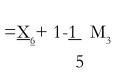
M4 = M3+X6-X1
5
If, X1 is not available for some reason, then we could substitute M3 for X1 as we known that the former was based on X1as well. The use of M3 as a substitute for X1Coould gives us a ‘best estimate of X1
M*4 = M3+X6-X
5
Where M*4 is used as an estimate of M4. This can be shown symbolically as follows:-
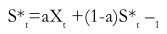
Where a varies between 0 and 1 and in the above example it is 1/5or02.
In case there are very small fluctuations in the time series, than we would like a to be small so as to maintain the effect of earlier data. However, in case of wide fluctuations a should be large so that our forecast is more realistic on account of its being responsive to these changes.
The main difficulty in exponential smoothing is how to ascertain the value of a. where using this method, it is advisable to try out several values of a and ascertain the extent of forecast error in each case. The value of a which gives the minimum forecast error should be then chosen for smoothing the time-series. This method consists of measuring the four components of a time series (i) trend, (ii) cycle, (iii) season, and (iv) erratic movement. The trend competent indicates long term effects on sales the are caused by such factors as income, population, industrialization the technology. The time period for a trend function varies considerably from a business cycle (which averages at 4-5 years).
The cyclical component indicates some sort of a periodicity in the general economic activity. When the data are plotted, they yield a curve with peaks and troughs, indicating and falls in the given series with a certain periodicity. A careful study of the impact of a business cycle must be made on the sale of each product. Cyclical forecasts are likely to be more accurate for the long term than for the short term. The seasonal component reflects changes in sales levels due to factors such as weather, festivals, holidays, etc. There is consistent reflects changes in sales levels due to factors such as weather, festivals, holidays, etc. there is a consistent pattern of sales for period within a year. Finally the erratic movements in data arise on account of events such as strikes, lockouts, price wars, etc. the decomposition of time enable identification of events such as sticks, lockouts, price wars, etc. the decomposition of time series enables of the error component from the trend, cycle and season which are systematic components.
Causal or Explanatory Methods: Causal or explanatory methods are regarded as the most sophisticated methods of forecasting sales. These methods yield realistic relevant data are available on the major variables influencing changes in sales. There are three advantages of causal methods. First, turning points in sales can be predicted more accurately by these methods than by time-series methods. Second, the use of these methods reduces the magnitude of the random component far more than it may be possible with the time series methods. Third, the use of such methods provides greater insight into causal relationships. This facilitates the management in marketing decision making. Isolated sales forecasts on the basis of time series methods would not be helpful in this regard.
Casual methods can be either (i) leading indicators or (ii) regression models. These are briefly discussed here.
Leading Indicators: Sometimes one finds that changes in sales of a particular product or service are preceded by changes in one or move leading indicators. In such cases, it is necessary to identify indicators and to closely observe changes in them. One example of a leading indicator is the demand for various household appliances which follows the construction of new houses. Likewise, the demand for many durables is preceded by an increase in disposable income. Yet another example is of number of births. The demand for baby food and other goods needed by infants can be ascertained by the number of births in a territory. It may be possible to include leading indicators in regression models.
Regression Models: Linear regression analysis is perhaps the most frequently used and the most powerful method among causal methods.
First, regression models indicate linear relationships within the range of observations and at the times when they were made. For example, if a regression analysis of sales is attempted on the basis of independent variables of population sizes of 15 million to 30 million and per capita income of Rs 1000 to Rs 2500, the regression model shows the relationships that existed between these extremes in the two independent variables. If the sales forecast is to be made on the basis of values of independent variables falling outside the above ranges, then the relationships expressed by the regression model may not hold good. Second, sometimes there may be a legged relationship between the dependent and independent variables. In such cases, the values of dependent variables are to be related to those of independent variables for the preceding month or year as the case may be. The search for factors with a lead lag relationship to the sales of a particular product is rather difficult. One should try out several indicators before selecting the one which is most satisfactory. Third, it may happen that the data required to establish the ideal relationship, do not exist or are inaccessible or, if available, are not useful. Therefore, the researcher has to be careful in using the data. He should be quire familiar with the varied sources and types of data that can be used in forecasting. He should also know about their strengths and limitations. Finally, regression model reflects the association among variables. The causal interpretation is done by the researcher on the basis of his understanding of such an association. As such, he should be extremely careful in choosing the variables so that a real causative relationship can be established among the variables chosen.
Input – Output Analysis: Another method that is widely used for forecasting is the input –output analysis. Here, the researcher takes into consideration a large number of factors, which affect the outputs which affect the outputs he is trying to forecast. For this purpose, an input – output table is prepaid where the inputs are shown horizontally as the column headings and outputs vertically as the stubs. It may be mentioned that by themselves input-output flows are of little direct use to the researcher. It is the application of an assumption as to how the output of an industry is related to its use of various inputs that makes an input-output analysis a good method of forecasting. The assumption states that as the level of an industry have output changes, the use of inputs will change proportionately, implying that there is no substitution in production among the various inputs. This may or may not hold good.
The use of input-output analysis in sales forecasting is appropriate for products sold to governmental, institutional and industrial marks as they have district patterns of usage. It is seldom used for consumer products and services. It would be most appropriate when the levels and kinds of inputs required to achieve certain levels of outputs need to be known.
A major constraint in the use of this method is that it needs extensive data for a large number of items which may not be easily available. Large business organizations may be in a position to collect such data on a continuing basis so that they can use input-output analysis for forecasting. However, that is not possible in case of small industrial organizations on account of excessive costs involved in the collection of comprehensive data. It is for this reason that input-output analysis is less widely used than most analysis initially expected.
Econometric Model: Econometric is concerned with the use of statistical and mathematical techniques to verify hypotheses emerging in economic theory.” An econometric model incorporates functional relationships estimated by these techniques into an internally consistent and logically self contained framework.” Econometric models use both exogenous and endogenous variables. Exogenous variables are used as inputs into the system but they themselves are determined outside the model. These variables include policy variables and uncontrolled events. In contrast, endogenous variables are those which are determined within the system.
The use of econometric models is generally found at the macro level such as forecasting national income and its components. Such models show how the economy or any of its specific segment operates. As compared to an ordinary regression equation they bring out the causalities involved more distinctly. This merit of econometric models enables them to predict turning points more accurately. However, their use at the micro-level for forecasting has so far been extremely limited.
Manager’s Guide to Forecasting: It may be noted that each method has strengths and weaknesses and every forecasting situation is subjected to constraints like time, competence or data. It is, therefore, necessary balance the advantages and limitations of forecasting methods in relation to the limitations and requirements of a situation to be forecast. This is an extremely difficult task which the management has to perform.
Manager should be given broad guidelines to help them decided on the most appropriate forecasting method. David M. Gorgoff and Robert G. Murdick have developed a chart that groups and profiles as many as 20 forecasting methods and arrays them against 16 important evaluative dimensions. Their chart can be useful to managers in two ways. The first is in selecting the best possible method for a given forecasting situations. The second is in deciding two to combine two or more forecasting methods to obtain batter forecasts.
There are several important factors which must be considered by managers before they finally decide to use a particular forecasting method. These are briefly discussed below.
Time Horizon: One reason why this is important is that the relative importance of different sub patterns changes as the time horizon of planning changes. Thus, in the immediate term, the randomness: in the short term, the seasonal factor; in the medium term, the cyclical component; and in the long term, and trend component ; dominate. Normally managers would like the forecast results to extend as far as possible into the future. However, if the period is too long, there are likely to be more complexities in the selection of proper forecasting techniques. It is because of this fact that some techniques are more suitable in a short span of time while others are not.
Technical Sophistication: Manager may have to improve their skills in understanding the forecast results generated through the use of advanced computers and mathematic.
Cast: There are three main elements of cost in a forecasting technique: development costs, data storage costs and costs of repeated applications. The relative importance of these elements varies with the technique of forecasting as well as the situation. A technique which is extremely costly may not be used even if it gives better forecasts. A point worth noting is that the cost of any method is more important at the beginning when it is being developed and installed.
Data Availability: it is advisable for the manger to ensure that the data needed by a particular forecasting method are available and reliable. Sometimes one may find that a particular method needs extensive data that are not available.
Variability and Consistency of Data: Like the availability of data, the manager must also satisfy himself regarding the variability and consistency of data to be used in a forecasting method. In case the company expects a change to take place in some established relationship, the forecaster may apply his judgment in a quantitative method. Alternatively, it may be advisable to use a qualitative method of forecasting.
Amount of Detail Necessary: Very often managers have to determine sales quotas or allocate resources to different territories. In such cases, aggregate forecasts alone are not sufficient. In view of this, managers may go in for a forecasting method that can first accurately predict individual components which can be combined subsequently into an overall for east.
Accuracy: The managers must aim at maximum accuracy of the forecast, and in the majority of forecasting situations accuracy is indeed regarded the most important criterion for selecting a forecasting technique. It may also be noted that some other are also frequently reflected in accuracy. For example, a less accurate forecast may be due to inadequate data or an inappropriate technique. Although there is no single universally accepted measure of accuracy, the following method is commonly used : Where MSE is the mean squared error ; Xi is the actual value; Fi is the forecast and n is the number of data values. It can be seen that the lower the value of MSE, the more accurate the forecast.
Turning Points: since turning points represent periods of exceptional opportunity or caution, the manager should examine whether a particular method is able to anticipate basic shifts. Here the manager has to be careful and identify methods which might give misleading signals for fundamental shifts.
Form: The form of a forecast varies considerably. Manager should prefer a method that gives some sort of central value and a range of possible outcomes. Arrange of forecasts comprising a high and a low figure may be more helpful to managers in determining the extent or risk, expected outcomes and most likely distributions.
It is true that even some quantitative forecasts involve an element of subjectivity. However, manager should be guided more by quantitative methods of forecasting rather by their own judgment. It has been well established by research on forecasting that quantitative methods are superior to the unstructured intuitive assessments of experts. Further, adjusting values of a quantitatively derived forecast on the basis of intuition or judgment of the manager will reduce the accuracy of such a forecast. Accordingly intention or judgment should be resorted to sparingly when there is sufficient justification to do so.
Finally, the task of forecasting should not be exclusively entrusted to a single person. While it should by one pensions, preferably the marketing research manager, such key people as sales managers and production managers must be actively involved in it. It is important to ensure that there is a consensus for a particular forecast. In the absence of it, the forecast is not likely to be taken seriously and, as a result, its utility will be much less.
