The sales volume which equates total revenue with related costs and results in neither profit nor loss is called break-even point (BEP). Break-even point can be determined by the following methods:
Algebraic methods:
- Contribution Margin Approach
- Equation technique
Graphic presentation:
- Break-even chart
- Profit volume chart
Algebraic Methods
Contribution Margin Approach
Equation Technique
It is based on an income equation i.e.
Sales – Total costs = Net profit.
Breaking up total costs into fixed and variable,
Sales – Fixed costs – Variable cost = Net profit
Sales = Fixed costs + Variable cost + Net profit
i.e.
SP(S) = FC + VC(S) + P
where
SP = Selling price per unit
S = Number of units required to be sold to break-even
FC = Total fixed costs
VC = Variable cost per unit
P = Net profit (Zero)
SP(S) = FC + VC(S) + Zero
SP(S) = FC + VC(S) + 0
SP(S) – VC(S) = FC
or
S(SP – VC) = FC
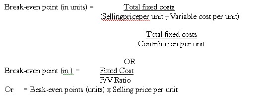
S = FC / (SP−VC )
To calculate the level of sales required to earn a particular level of profit, the formula is:
Required Sales (in) = (Fixed cost +Desired profit_ / P/V Ratio
Graphic Presentation
Break-even chart
According to the Chartered Institute of Management Accountants, London the break-even chart means “a chart which shows profit or neither loss at various levels of activity, the level at which neither profit nor loss is shown being termed as the break-even point”.
It is a graphic relationship between costs, volume and profits. It shows not only the BEP but also the effects of costs and revenue at varying levels of sales. The break-even chart can therefore, be more appropriately called the cost-volume-profit graph.
Assumptions regarding Break-Even Charts are as under:
- Costs are bifurcated into variable and fixed components.
- Fixed costs will remain constant and will not change with change in level of output.
- Variable cost per unit will remain constant during the relevant volume range of graph.
- Selling price will remain constant even though there maybe competition or change in volume of production.
- The number of units produced and sold will be the same so that there is no operating or closing stock.
- There will be no change in operating efficiency.
- In case of multi-product companies, it is assumed that the sales mix remains constant.
A break-even chart can be presented in different forms.
First Method of Break even chart
On the X-axis of the graph is plotted the volume of productions or the quantities of sales and on the Y-axis (vertical line) costs and sales revenues are represented. The fixed costs line is drawn parallel to X-axis. The variable costs for different levels of activity are plotted over the fixed cost line, which shows that the cost is increasing with the increase in the volume of output. The variable cost line is joined to fixed cost line at zero volume of production. This line is regarded as the total cost line. Sales values at various levels of output are plotted from the origin and joined is called the sales line. The sales line will cut the total cost line at a point where the total costs equal to total revenues and this point of intersection of two lines is known as break-even point or the point of no profit no loss. The lines produced from the inter-section to Y-axis and X-axis may give sales value and the number of units produced at break-even point respectively. Loss and profit are as have been shown in the chart which shows that if production is less than the break-even point, the business shall be running at a loss and if the production is more than the breakeven level, there will be profit. The angle which the sales line makes with total cost line while intersecting it at BEP is called angle of incidence. A large angle of incidence denotes a good profit position of a company.
Illustration 2
From the following data, calculate the break-even point by means of a break-even chart:
Selling price per unit Variable cost per unit Total fixed cost
Solution:
Selling price per unit = 15
Variable cost per unit = 10
Total fixed cost = 1,50,000
For plotting the data, we need at least two points – one for plotting the total cost line and other for plotting the total sales line. Therefore, it will be necessary to presume different levels of output and sales as below:
Second Method of Break even chart
This is variation of the first method in which variable cost line is drawn first and thereafter drawing the fixed cost line above the variable cost line. The later line will be the total cost line. The sales line is drawn as usual. The added advantage of this method is that contributions at various levels of output are automatically depicted in the chart.
Contribution break-even chart: The chart helps in ascertaining the amount of contribution at different levels of activity besides the break-even point. In this method, the fixed cost line is drawn parallel to the X-axis. The contribution line is then drawn from the origin which goes up with the increase in output. The sales line is plotted as usual, but the question of intersection of sales line with cost line does not arise. The contribution line crosses the fixed cost line and the point of intersection is treated as break-even point. At this point, contribution is equal to fixed expenses and there is no profit or loss. If the contribution is more than the fixed expenses, profit will arise and if the contribution is less than the fixed expenses, loss will arise.
Profit-volume Graph: Profit volume graph is the graphical representation of the relationship between profit and volume. Separate lines for costs and revenues are eliminated from the P/V graph as only profit points are plotted. It is based on the same information as is required for the traditional break-even chart and is characterized by the same limitations. The steps in the construction of profit volume graph are as follows:
- Profit and fixed costs are represented on the vertical axis.
- Sales are shown on the horizontal axis.
- The sale line divides the graph into two parts both horizontally and vertically. The area above the horizontal line is the ‘profit area’ and that below it is the ‘loss area’ at which fixed costs are represented on the vertical axis below the sale line and profits on the same axis above the sale line.
- Profits and fixed costs are plotted for corresponding sales volume and the points are joined by a line which is the profit line.
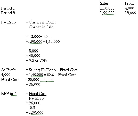
Illustration 5
Sales are 1, 50,000, producing a profit of 4,000 in period I. Sales are 1,90,000, producing a profit of 12,000 in period II. Determine the BEP.
Solution:
The Question may be presented in the given format: