The farthest one can reduce a set of data, and still retain any information at all, is to summarize the data with a single value. Measures of location do just that: They try to capture with a single number what is typical of the data. What single number is most representative of an entire list of numbers? We cannot say without defining “representative” more precisely. We will study three common measures of location: the mean, the median, and the mode. The mean, median and mode are all “most representative,” but for different, related notions of representativeness.
For qualitative and categorical data, the mode makes sense, but the mean and median do not.
It is hard to see the connection between the mean, median, and mode from their definitions.
However, the mean, the median, and the mode are “as close as possible” to all the data: For each of these three measures of location, the sum of the distances between each datum and the measure of location is as small as it can be. The differences among the three measures of location are in how “distance” is defined.
- For the mean, the distance between two numbers is defined to be the square of their difference. That is, the sum of the squares of the differences between the data and the mean is smaller than the sum of squares of the differences between the data and any other number. (Equivalently, the rms or root mean square of the differences from the mean is smaller than the rms of the list of differences from any other number.)
- For the median, the distance between two numbers is defined to be the absolute value of their difference. That is, the sum of the absolute values of the differences between a median and the data is no larger than the sum of the absolute values of the differences between any other number and the data.
- For the mode, the distance between two numbers is defined to be zero if the numbers are equal, and one if they are not equal. That is, the number of data that differ from a mode is no larger than the number of data that differ from any other value. Equivalently, a mode is a number from which the fewest possible data differ: a “most common” value.
The mean, median, and mode can be related (approximately) to the histogram: loosely speaking, the mode is the highest bump, the median is where half the area is to the right and half is to the left, and the mean is where the histogram would balance, were it a solid object cut out of a uniform block of metal. (All these heuristics are approximate, and depend on the class intervals.)
Central Tendencies – Central tendency is a measure that characterizes the central value of a collection of data that tends to cluster somewhere between the high and low values in the data. It refers to measurements like mean, median and mode. It is also called measures of center. It involves plotting data in a frequency distribution which shows the general shape of the distribution and gives a general sense of how the numbers are grouped. Several statistics can be used to represent the “center” of the distribution.
Mean
The mean is the most common measure of central tendency. It is the ratio of the sum of the scores to the number of the scores. For ungrouped data which has not been grouped in intervals, the arithmetic mean is the sum of all the values in that population divided by the number of values in the population as

where, µ is the arithmetic mean of the population, Xi is the ith value observed, N is the number of items in the observed population and ∑ is the sum of the values. For example, the production of an item for 5 days is 500, 750, 600, 450 and 775 then the arithmetic mean is µ = 500 + 750 + 600 + 450 + 775/ 5 = 615. It gives the distribution’s arithmetic average and provides a reference point for relating all other data points. For grouped data, an approximation is done using the midpoints of the intervals and the frequency of the distribution as

Weighted Mean – When a mean is calculated, a serious mistake can be committed if one overlooks the fact that the quantities that are being averaged are not all of equal importance with reference to the situation being described. Consider, for example, a cruise line that advertises the following fares for single-occupancy cabins on an 11-day cruise
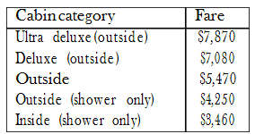
The mean of these five fares is
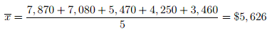
But one cannot very well say that the average fare for one of these single occupancy cabins is $5,626. To get that figure, we would also have to know how many cabins there are in each of the categories. Referring to the ship’s deck plan, where the cabins are color-coded by category, an analyst finds that there are, respectively, 6, 4, 8, 13, and 22 cabins available in these five categories. If it can be assumed that these 53 cabins will all be occupied, the cruise line can expect to receive a total of
6(7, 870) + 4(7, 080) + 8(5, 470) + 13(4, 250) + 22(3, 460) = 250, 670
for the 53 cabins and, hence, on the average
To give quantities being averaged their proper degree of importance, it is necessary to assign them relative importance weights and then calculate a weighted mean. In general, the weighted mean xw of a set of numbers x1, x2, x3, . . . and xn, whose relative importance is expressed numerically by a corresponding set of numbers w1, w2, w3, . . . and wn is given by:
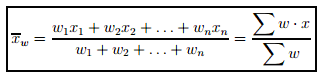
Here Ʃw is the sum of the products obtained by multiplying each x by the corresponding weight, and Ʃw is simply the sum of the weights. Note that when the weights are all equal, the formula for the weighted mean reduces to that for the ordinary (arithmetic) mean.
Median
It divides the distribution into halves; half are above it and half are below it when the data are arranged in numerical order. It is also called as the score at the 50th percentile in the distribution. The median location of N numbers can be found by the formula (N + 1) / 2. When N is an odd number, the formula yields an integer that represents the value in a numerically ordered distribution corresponding to the median location. (For example, in the distribution of numbers (3 1 5 4 9 9 8) the median location is (7 + 1) / 2 = 4. When applied to the ordered distribution (1 3 4 5 8 9 9), the value 5 is the median. If there were only 6 values (1 3 4 5 8 9), the median location is (6 + 1) / 2 = 3.5 hence, median is half-way between the 3rd and 4th scores (4 and 5) or 4.5. It is the distribution’s center point or middle value with an equal number of data points occur on either side of the median but useful when the data set has extreme high or low values and used with non-normal data
Mode
It is the most frequent or common score in the distribution or the point or value of X that corresponds to the highest point on the distribution. If the highest frequency is shared by more than one value, the distribution is said to be multimodal and with two, it is bimodal or peaks in scoring at two different points in the distribution. For example in the measurements 75, 60, 65, 75, 80, 90, 75, 80, 67, the value 75 appears most frequently, thus it is the mode.
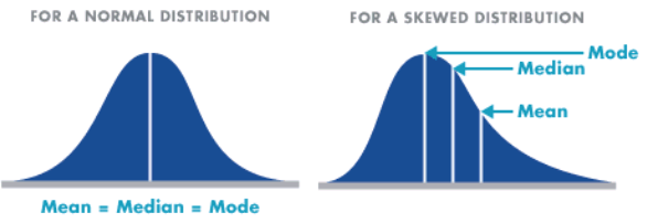
In general, the mean and the median need not be close together. If the data have a symmetric distribution, the mean and median are exactly equal, but if the distribution of the data is skewed, the difference between mean and the median can be large. This is because data in the tails of the distribution have a lot of leverage on the mean, just as a light person can balance a much heavier one on a see-saw if she sits much farther from the fulcrum than the heavier person does. The median is smaller than the mean if the data are skewed to the right, and larger than the mean if the data are skewed to the left.