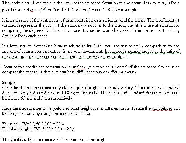
A measure of spread, sometimes also called a measure of dispersion, is used to describe the variability in a sample or population. It is usually used in conjunction with a measure of central tendency, such as the mean or median, to provide an overall description of a set of data.
There are many reasons why the measure of the spread of data values is important, but one of the main reasons regards its relationship with measures of central tendency. A measure of spread gives us an idea of how well the mean, for example, represents the data. If the spread of values in the data set is large, the mean is not as representative of the data as if the spread of data is small. This is because a large spread indicates that there are probably large differences between individual scores. Additionally, it is often seen as positive if there is little variation in each data group as it indicates that they are similar. The averages are representatives of a frequency distribution. But they fail to give a complete picture of the distribution. They do not tell anything about the scatterness of observations within the distribution.
Although the average value in a distribution is informative about how scores are centered in the distribution, the mean, median, and mode lack context for interpreting those statistics.
If the data is clustered around the center value, the “spread” is small. The further the distances of the data values from the center value, the greater the “spread”.
Measures of variability provide information about the degree to which individual scores are clustered about or deviate from the average value in a distribution.
Range
The simplest measure of variability to compute and understand is the range. The range is the difference between the highest and lowest score in a distribution. Although it is easy to compute, it is not often used as the sole measure of variability due to its instability. Because it is based solely on the most extreme scores in the distribution and does not fully reflect the pattern of variation within a distribution, the range is a very limited measure of variability. The range is based on only two values within the set, which may tell very little about “how” the remaining values are distributed in the set. For this reason, range is used as a supplement to other measures of spread, instead of being the only measure of spread.
For example, let us consider the following data set:
23 56 45 65 59 55 62 54 85 25
The maximum value is 85 and the minimum value is 23. This results in a range of 62, which is 85 minus 23. Whilst using the range as a measure of spread is limited, it does set the boundaries of the scores. This can be useful if you are measuring a variable that has either a critical low or high threshold (or both) that should not be crossed. The range will instantly inform you whether at least one value broke these critical thresholds. In addition, the range can be used to detect any errors when entering data. For example, if you have recorded the age of school children in your study and your range is 7 to 123 years old you know you have made a mistake!
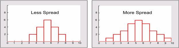
Inter-quartile Range (IQR)
It divides the set into four equal parts (or quarters). The three values that form the four divisions are called quartiles: first quartile, Q1; second quartile (median), Q2, and third quartile, Q3. The interquartile range is the difference between the third quartile and the first quartile. You can think of the IQR (also called the midspread or middle fifty) as a “range” between the third and first quartiles. The IQR is considered a more stable statistic than the typical range of a data set, as seen in the first section. The IQR contains 50% of the data, eliminating the influence of outliers.
It provides a measure of the spread of the middle 50% of the scores. The IQR is defined as the 75th percentile – the 25th percentile. The interquartile range plays an important role in the graphical method known as the boxplot. The advantage of using the IQR is that it is easy to compute and extreme scores in the distribution have much less impact but its strength is also a weakness in that it suffers as a measure of variability because it discards too much data. Researchers want to study variability while eliminating scores that are likely to be accidents. The boxplot allows for this for this distinction and is an important tool for exploring data.
Quartiles tell us about the spread of a data set by breaking the data set into quarters, just like the median breaks it in half. For example, consider the marks of the 100 students below, which have been ordered from the lowest to the highest scores, and the quartiles highlighted in red.
Order Score Order Score Order Score Order Score Order Score
1st 35 21st 42 41st 53 61st 64 81st 74
2nd 37 22nd 42 42nd 53 62nd 64 82nd 74
3rd 37 23rd 44 43rd 54 63rd 65 83rd 74
4th 38 24th 44 44th 55 64th 66 84th 75
5th 39 25th 45 45th 55 65th 67 85th 75
6th 39 26th 45 46th 56 66th 67 86th 76
7th 39 27th 45 47th 57 67th 67 87th 77
8th 39 28th 45 48th 57 68th 67 88th 77
9th 39 29th 47 49th 58 69th 68 89th 79
10th 40 30th 48 50th 58 70th 69 90th 80
11th 40 31st 49 51st 59 71st 69 91st 81
12th 40 32nd 49 52nd 60 72nd 69 92nd 81
13th 40 33rd 49 53rd 61 73rd 70 93rd 81
14th 40 34th 49 54th 62 74th 70 94th 81
15th 40 35th 51 55th 62 75th 71 95th 81
16th 41 36th 51 56th 62 76th 71 96th 81
17th 41 37th 51 57th 63 77th 71 97th 83
18th 42 38th 51 58th 63 78th 72 98th 84
19th 42 39th 52 59th 64 79th 74 99th 84
20th 42 40th 52 60th 64 80th 74 100th 85
The first quartile (Q1) lies between the 25th and 26th student’s marks, the second quartile (Q2) between the 50th and 51st student’s marks, and the third quartile (Q3) between the 75th and 76th student’s marks. Hence:
First quartile (Q1) = 45 + 45 ÷ 2 = 45
Second quartile (Q2) = 58 + 59 ÷ 2 = 58.5
Third quartile (Q3) = 71 + 71 ÷ 2 = 71
In the above example, we have an even number of scores (100 students, rather than an odd number, such as 99 students). This means that when we calculate the quartiles, we take the sum of the two scores around each quartile and then half them (hence Q1= 45 + 45 ÷ 2 = 45) . However, if we had an odd number of scores (say, 99 students), we would only need to take one score for each quartile (that is, the 25th, 50th and 75th scores). You should recognize that the second quartile is also the median.
Quartiles are a useful measure of spread because they are much less affected by outliers or a skewed data set than the equivalent measures of mean and standard deviation. For this reason, quartiles are often reported along with the median as the best choice of measure of spread and central tendency, respectively, when dealing with skewed and/or data with outliers. A common way of expressing quartiles is as an interquartile range. The interquartile range describes the difference between the third quartile (Q3) and the first quartile (Q1), telling us about the range of the middle half of the scores in the distribution. Hence, for our 100 students:
Interquartile range = Q3 – Q1
= 71 – 45
= 26
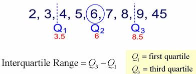
Variance (s2)
The variance is a measure based on the deviations of individual scores from the mean. As, simply summing the deviations will result in a value of 0 hence, the variance is based on squared deviations of scores about the mean. When the deviations are squared, the rank order and relative distance of scores in the distribution is preserved while negative values are eliminated. Then to control for the number of subjects in the distribution, the sum of the squared deviations, is divided by N (population) or by N – 1 (sample). The result is the average of the sum of the squared deviations and it is called the variance. The variance is not only a high number but it is also difficult to interpret because it is the square of a value.
The variance achieves positive values by squaring each of the deviations instead. Adding up these squared deviations gives us the sum of squares, which we can then divide by the total number of scores in our group of data
As a measure of variability, the variance is useful. If the scores in our group of data are spread out, the variance will be a large number. Conversely, if the scores are spread closely around the mean, the variance will be a smaller number. However, there are two potential problems with the variance. First, because the deviations of scores from the mean are ‘squared’, this gives more weight to extreme scores. If our data contains outliers (in other words, one or a small number of scores that are particularly far away from the mean and perhaps do not represent well our data as a whole), this can give undo weight to these scores. Secondly, the variance is not in the same units as the scores in our data set: variance is measured in the units squared. This means we cannot place it on our frequency distribution and cannot directly relate its value to the values in our data set.
A small variance indicates that the data points tend to be very close to the mean and to each other A high variance indicates that the data points are very spread out from the mean and from each other. One problem with the variance is that it does not have the same unit of measure as the original data.
Process
- Find the mean (average) of the set.
- Subtract each data value from the mean to find its distance from the mean.
- Square all distances.
- Add all the squares of the distances. Divide by the number of pieces of data (for population variance).
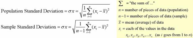
Standard deviation (s)
The standard deviation is defined as the positive square root of the variance and is a measure of variability expressed in the same units as the data. The standard deviation is very much like a mean or an “average” of these deviations.
The standard deviation is a measure of the spread of scores within a set of data. Usually, we are interested in the standard deviation of a population. However, as we are often presented with data from a sample only, we can estimate the population standard deviation from a sample standard deviation. These two standard deviations – sample and population standard deviations – are calculated differently. In statistics, we are usually presented with having to calculate sample standard deviations
In a normal (symmetric and mound-shaped) distribution, about two-thirds of the scores fall between +1 and -1 standard deviations from the mean and the standard deviation is approximately 1/4 of the range in small samples (N < 30) and 1/5 to 1/6 of the range in large samples (N > 100).
A low standard deviation indicates that the data points tend to be very close to the mean. A high standard deviation indicates that the data points are spread out over a large range of values.
The standard deviation is a measure of the spread of scores within a set of data. Usually, we are interested in the standard deviation of a population. However, as we are often presented with data from a sample only, we can estimate the population standard deviation from a sample standard deviation. These two standard deviations – sample and population standard deviations – are calculated differently. In statistics, we are usually presented with having to calculate sample standard deviations.
We are normally interested in knowing the population standard deviation because our population contains all the values we are interested in. Therefore, you would normally calculate the population standard deviation if: (1) you have the entire population or (2) you have a sample of a larger population, but you are only interested in this sample and do not wish to generalize your findings to the population. However, in statistics, we are usually presented with a sample from which we wish to estimate (generalize to) a population, and the standard deviation is no exception to this. Therefore, if all you have is a sample, but you wish to make a statement about the population standard deviation from which the sample is drawn, you need to use the sample standard deviation. Confusion can often arise as to which standard deviation to use due to the name “sample” standard deviation incorrectly being interpreted as meaning the standard deviation of the sample itself and not the estimate of the population standard deviation based on the sample.
The standard deviation is used in conjunction with the mean to summarise continuous data, not categorical data. In addition, the standard deviation, like the mean, is normally only appropriate when the continuous data is not significantly skewed or has outliers.
Usage Examples
Example 1 – A teacher sets an exam for their pupils. The teacher wants to summarize the results the pupils attained as a mean and standard deviation. Which standard deviation should be used?
Population standard deviation. Why? Because the teacher is only interested in this class of pupils’ scores and nobody else.
Example 2 – A researcher has recruited males aged 45 to 65 years old for an exercise training study to investigate risk markers for heart disease (e.g., cholesterol). Which standard deviation would most likely be used?
Sample standard deviation. Although not explicitly stated, a researcher investigating health related issues will not simply be concerned with just the participants of their study; they will want to show how their sample results can be generalised to the whole population (in this case, males aged 45 to 65 years old). Hence, the use of the sample standard deviation.
Example 3 – One of the questions on a national consensus survey asks for respondents’ age. Which standard deviation would be used to describe the variation in all ages received from the consensus?
Population standard deviation. A national consensus is used to find out information about the nation’s citizens. By definition, it includes the whole population. Therefore, a population standard deviation would be used.
Sample
Discrete Distribution Question – The weights of 5 ear-heads of sorghum are 100, 102,118,124,126 gms. Find the standard deviation.
Solution
| x | x2 |
| 100 | 10000 |
| 102 | 10404 |
| 118 | 13924 |
| 124 | 15376 |
| 126 | 15876 |
| 570 | 65580 |
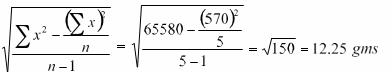
Standard Deviation =
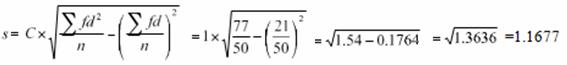
Continuous Distribution Question – The Frequency distributions of seed yield of 50 sesame plants are given below. Find the standard deviation.
| Seed yield in gms (x) | 2.5-35 | 3.5-4.5 | 4.5-5.5 | 5.5-6.5 | 6.5-7.5 |
| No. of plants (f) | 4 | 6 | 15 | 15 | 10 |
Solution
| Seed yield in gms (x) | No. of Plants f | Mid x | d= (x-A)/c | df | d2 f |
| 2.5-3.5 | 4 | 3 | -2 | -8 | 16 |
| 3.5-4.5 | 6 | 4 | -1 | -6 | 6 |
| 4.5-5.5 | 15 | 5 | 0 | 0 | 0 |
| 5.5-6.5 | 15 | 6 | 1 | 15 | 15 |
| 6.5-7.5 | 10 | 7 | 2 | 20 | 40 |
| Total | 50 | 25 | 0 | 21 | 77 |
A=Assumed mean = 5
n=50, C=1
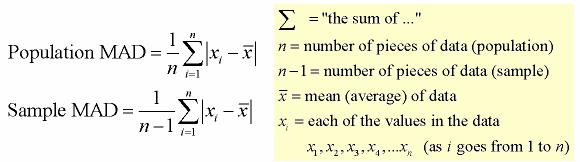
Mean Absolute Deviation (MAD)
The mean absolute deviation is the average (mean) of the absolute value of the differences between each piece of data in the data set and the mean of the set. It measures the average distances between each data element and the mean.
Process
- Find the mean (average) of the set.
- Subtract each data value from the mean to find its distance from the mean.
- Turn all distances to positive values (take the absolute value).
- Add all of the distances. Divide by the number of pieces of data (for population MAD).
It is the mean of the distances of each value from their mean. It is a robust measure of the variability of a univariate sample of quantitative data. It can also refer to the population parameter that is estimated by the MAD calculated from a sample.
Consider the data (1, 1, 2, 2, 4, 6, 9). It has a median value of 2. The absolute deviations about 2 are (1, 1, 0, 0, 2, 4, 7) which in turn have a median value of 1 (because the sorted absolute deviations are (0, 0, 1, 1, 2, 4, 7)). So the median absolute deviation for this data is 1.
Measures of variability can not be compared like the standard deviation of the production of bolts to the availability of parts. If the standard deviation for bolt production is 5 and for availability of parts is 7 for a given time frame, it can not be concluded that the standard deviation of the availability of parts is greater than that of the production of bolts thus, variability is greater with the parts. Hence, a relative measure called the coefficient of variation is used.