An association is any relationship between two measured quantities that renders them statistically dependent. The term “association” is closely related to the term “correlation.” Both terms imply that two or more variables vary according to some pattern. However, correlation is more rigidly defined by some correlation coefficient which measures the degree to which the association of the variables tends to a certain pattern.
It provides information about the relatedness between variables so as to help estimate the existence of a relationship between variables and it’s strength.
Most measures of association are scaled so that they reach a maximum numerical value of 1 when the two variables have a perfect relationship with each other. They are also scaled so that they have a value of 0 when there is no relationship between two variables. While there are exceptions to these rules, most measures of association are of this sort. Some measures of association are constructed to have a range of only 0 to 1, other measures have a range from -1 to +1. The latter provide a means of determining whether the two variables have a positive or negative association with each other.
Covariance
Variables are positively related if they move in the same direction. Variables are inversely related if they move in opposite directions.
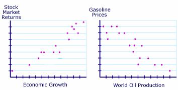
You are probably already familiar with statements about covariance that appear in the news almost daily. For example, you might hear that as economic growth increases, stock market returns tend to increase as well. These variables are said to be positively related because they move in the same direction. You may also hear that as world oil production increases, gasoline prices fall. These variables are said to be negatively, or inversely, related because they move in opposite directions.
The relationship between two variables can be illustrated in a graph. In the examples below, the graph on the left illustrates how the positive relationship between economic growth and market returns might appear. The graph indicates that as economic growth increases, stock market returns also increase. The graph on the right is an example of how the inverse relationship between oil production and gasoline prices might appear. It illustrates that as oil production increases, gas prices fall.
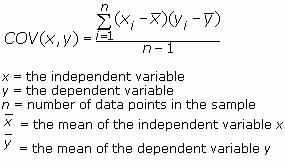
Covariance shows how the variable y reacts to a variation of the variable x. Its formula is for a population cov( X, Y ) = ∑( xi − µx) (yi − µy) / N
Formula for sample is as
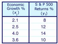
Consider the table below, which describes the rate of economic growth (xi) and the rate of return on the S&P 500 (yi).
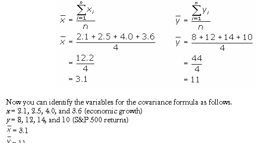
Using the covariance formula, you can determine whether economic growth and S&P 500 returns have a positive or inverse relationship. Before you compute the covariance, calculate the mean of x and y.
Substitute these values into the covariance formula to determine the relationship between economic growth and S&P 500 returns.
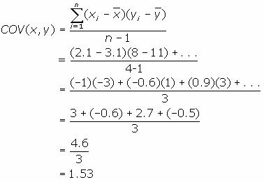
The covariance between the returns of the S&P 500 and economic growth is 1.53. Since the covariance is positive, the variables are positively related—they move together in the same direction.
Correlation coefficient (r)
Pearson’s correlation coefficient is the covariance of the two variables divided by the product of their standard deviations.
The quantity r, called the linear correlation coefficient, measures the strength and the direction of a linear relationship between two variables. The linear correlation coefficient is sometimes referred to as the Pearson product moment correlation coefficient in honor of its developer Karl Pearson. The mathematical formula for computing r is
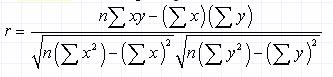
where n is the number of pairs of data.
The value of r is such that -1 < r < +1. The + and – signs are used for positive linear correlations and negative linear correlations, respectively.
- Positive correlation: If x and y have a strong positive linear correlation, r is close to +1. An r value of exactly +1 indicates a perfect positive fit. Positive values indicate a relationship between x and y variables such that as values for x increases, values for y also increase.
- Negative correlation: If x and y have a strong negative linear correlation, r is close to -1. An r value of exactly -1 indicates a perfect negative fit. Negative values indicate a relationship between x and y such that as values for x increase, values for y decrease.
- No correlation: If there is no linear correlation or a weak linear correlation, r is close to 0. A value near zero means that there is a random, nonlinear relationship between the two variables
- A perfect correlation of ± 1 occurs only when the data points all lie exactly on a straight line. If r = +1, the slope of this line is positive. If r = -1, the slope of this line is negative.
A correlation greater than 0.8 is generally described as strong, whereas a correlation less than 0.5 is generally described as weak. These values can vary based upon the “type” of data being examined.
r is a dimensionless quantity; that is, it does not depend on the units employed. It is a number that ranges between −1 and +1. The sign of r will be the same as the sign of the covariance. When r equals−1, then it is a perfect negative relationship between the variations of the x and y thus, increase in x will lead to a proportional decrease in y. Similarly when r equals +1, then it is a positive relationship or the changes in x and the changes in y are in the same direction and in the same proportion. If r is zero, there is no relation between the variations of both. Any other value of r determines the relationship as per how r is close to −1, 0, or +1. The formula for the correlation coefficient for population is ρ = Cov( X, Y ) /σx σy
Coefficient of determination (r2)
It measures the proportion of changes of the dependent variable y as explained by the independent variable x. It is the square of the correlation coefficient r thus, is always positive with values between zero and one. If it is zero, the variations of y are not explained by the variations of x but if it one, the changes in y are explained fully by the changes in x but other values of r are explained according to closeness to zero or one.
The coefficient of determination, r2, is useful because it gives the proportion of the variance (fluctuation) of one variable that is predictable from the other variable. It is a measure that allows us to determine how certain one can be in making predictions from a certain model/graph.
The coefficient of determination is the ratio of the explained variation to the total variation. The coefficient of determination is such that 0 < r 2 < 1, and denotes the strength of the linear association between x and y.
The coefficient of determination represents the percent of the data that is the closest to the line of best fit. For example, if r = 0.922, then r 2 = 0.850, which means that 85% of the total variation in y can be explained by the linear relationship between x and y (as described by the regression equation). The other 15% of the total variation in y remains unexplained. The coefficient of determination is a measure of how well the regression line represents the data. If the regression line passes exactly through every point on the scatter plot, it would be able to explain all of the variation. The further the line is away from the points, the less it is able to explain.
